☣

Probabilies & Statistics

TODO: @

《统计学习方法》
k-d tree - Wikipedia, the free encyclopedia
cart: classification and regression tree;, gini index

MISC Notes @

一个分布有 mean，一个随机变量有 ev。如果这个随机变量 rv 分布为 x，则 rv 的 ev 就是 x 的 mean。
说 chi-squared 和 chi-square，都可以, 维基上是 chi-squared，用这个比较好。
全概率：原因 -> 结果
贝叶斯：结果 -> 原因
P(A|B) > P(A), P(A|B) = P(A), P(A|B) < P(A)
相关（线性相关）
binomial, [baɪ'nomɪəl]
bernoulli, [bə:'nu:li]
poisson, /ˈpwɑːsɒn/
deviation, ['divɪ'eʃən]
cumulative, ['kjumjəletɪv]
均方误差（mean square error）
homoscedasticity, homo-sce-das-ti-city, 方差齐性, ['hɔməusi,dæs'tisəti]
fiducial, [fɪ'djuːʃ(ə)l]
bayesian, ['beʒən]
conjugate, ['kɑndʒəɡet], 共轭的

成对的；结合的；【化, 数, 物】共轭的；【语】同源 [根] 的 v.（根据数、人称、时态等）列举（动词）的变化形式
一些蛋疼的名词 @
An independent variable is also known as a “predictor variable”, “regressor”, “controlled variable”, “manipulated variable”, “explanatory variable”, “exposure variable” (see reliability theory), “risk factor” (see medical statistics), “feature” (in machine learning and pattern recognition) or an “input variable.”

A dependent variable is also known as a “response variable”, “regressand”, “predicted variable”, “measured variable”, “explained variable”, “experimental variable”, “responding variable”, “outcome variable”, and “output variable”.

“Explanatory variable” is preferred by some authors over “independent variable” when the quantities treated as “independent variables” may not be statistically independent. If the independent variable is referred to as an “explanatory variable” then the term “response variable” is preferred by some authors for the dependent variable.

“Explained variable” is preferred by some authors over “dependent variable” when the quantities treated as “dependent variables” may not be statistically dependent. If the dependent variable is referred to as an “explained variable” then the term “predictor variable” is preferred by some authors for the independent variable.

Variables may also be referred to by their form:
- continuous,
- binary/dichotomous,
- nominal categorical, and
- ordinal categorical, among others.
A variable may be thought to alter the dependent or independent variables, but may not actually be the focus of the experiment. So that variable will be kept constant or monitored to try to minimise its effect on the experiment. Such variables may be designated (指定) as either a “controlled variable”, “control variable”, or “extraneous variable”.

Extraneous variables, if included in a regression as independent variables, may aid a researcher with accurate response parameter estimation, prediction, and goodness of fit, but are not of substantive interest to the hypothesis under examination. For example, in a study examining the effect of post-secondary education on lifetime earnings, some extraneous variables might be gender, ethnicity, social class, genetics, intelligence, age, and so forth. A variable is extraneous only when it can be assumed (or shown) to influence the dependent variable. If included in a regression, it can improve the fit of the model. If it is excluded from the regression and if it has a non-zero covariance with one or more of the independent variables of interest, its omission will bias the regression’s result for the effect of that independent variable of interest. This effect is called confounding or omitted variable bias; in these situations, design changes and/or statistical control is necessary.

Extraneous variables are often classified into three types:
- Subject variables, which are the characteristics of the individuals being studied that might affect their actions. These variables include age, gender, health status, mood, background, etc.
- Blocking variables or experimental variables are characteristics of the persons conducting the experiment which might influence how a person behaves. Gender, the presence of racial discrimination, language, or other factors may qualify as such variables.
- Situational variables are features of the environment in which the study or research was conducted, which have a bearing on the outcome of the experiment in a negative way. Included are the air temperature, level of activity, lighting, and the time of day.
In quasi-experiments, differentiating between dependent and other variables may be downplayed in favour of differentiating between those variables that can be altered by the researcher and those that cannot.[citation needed] Variables in quasi-experiments may be referred to as “extraneous variables”, “subject variables”, “blocking variables”, “situational variables”, “pseudo-independent variables”, “ex post facto variables”, “natural group variables” or “non-manipulated variables”.

In modelling, variability that is not covered by the independent variable is designated by e_i and is known as the “residual”, “side effect”, “error”, “unexplained share”, “residual variable”, or “tolerance”.

refs and see also
- Dependent and independent variables - Wikipedia, the free encyclopedia

值得打印出来的“小抄”：Probability Cheatsheet

Probability theory @

Probability theory is the branch of mathematics concerned with probability, the analysis of random phenomena. The central objects of probability theory are random variables, stochastic processes, and events: mathematical abstractions of non-deterministic events or measured quantities that may either be single occurrences or evolve over time in an apparently random fashion.

Terminology (words) @

RV: Random Varible
CRV: Continuous Random Varaible
DRV: Discrete Random Varaible
CDF, joint CDF
PMF, joint PMF
PDF, joint PDF
EV: expected value
LOTUS: Law of the Unconscious Statistician
Indicator Random Variables
UoU: Universality of Uniform
MGF: Moment Generating Functions
CLT: Central Limit Theorem
LLN: Law of Large Numbers
RSS: Residual Sum of Squares
OLS, ordinary least square
LAD, Least absolute deviations, also known as least absolute errors (LAE),
stochastic [stə'kæstɪk] adj.【数】随机的；机会的；有可能性的；随便的, random error -> stochastic error.

Mode, mean, median @

Geometric visualisation of the mode, median and mean of an arbitrary probability density function.

才注意到这里 mean 表示成了一个天平一样的东西……

Moment (mathematics) @

In mathematics, a moment is a specific quantitative measure, used in both mechanics and statistics, of the shape of a set of points. If the points represent mass, then the zeroth moment is the total mass, the first moment divided by the total mass is the center of mass, and the second moment is the rotational inertia. If the points represent probability density, then the zeroth moment is the total probability (i.e. one), the first moment is the mean, the second central moment is the variance, the third moment is the skewness, and the fourth moment (with normalization and shift) is the kurtosis. The mathematical concept is closely related to the concept of moment in physics.

对于 bounded distribution，全部的矩决定了分布。

For a bounded distribution of mass or probability, the collection of all the moments (of all orders, from 0 to ∞) uniquely determines the distribution.

矩的定义（CRV）。 The n-th moment of a real-valued continuous function f(x) of a real variable about a value c is

\[\mu_n=\int_{-\infty}^\infty (x - c)^n\,f(x)\,dx.\]

For the second and higher moments, the central moments (moments about the mean, with c being the mean) are usually used rather than the moments about zero, because they provide clearer information about the distribution’s shape.

Other moments may also be defined. For example, the n-th inverse moment about zero is $\operatorname{E}\left[X^{-n}\right]$ and the n-th logarithmic moment about zero is $\operatorname{E}\left[\ln^n(X)\right]$.

Significance of moments (raw, central, standardised) and cumulants （累计误差） (raw, standardised), in connection with named properties of distributions:

mean

The first raw moment is the mean.
variance

The second central moment is the variance. Its positive square root is the standard deviation σ.
skewness

The third central moment is a measure of the lopsidedness (不平衡) of the distribution; any symmetric distribution will have a third central moment, if defined, of zero. The normalised third central moment is called the skewness, often γ (gamma).¹
Kurtosis

[kɜː'təʊsɪs] n.【统】峭度, 峰度；峰态；峰度系数
Normalised moments

The normalised n-th central moment or standardized moment is the n-th central moment divided by σn; the normalised n-th central moment of

\[x = \frac{\operatorname{E} \left [(x - \mu)^n \right ]}{\sigma^n}.\]

Standard error @

The standard error (SE) is the standard deviation of the sampling distribution of a statistic, most commonly of the mean. The term may also be used to refer to an estimate of that standard deviation, derived from a particular sample used to compute the estimate.

For a value that is sampled with an unbiased normally distributed error, the above depicts the proportion of samples that would fall between 0, 1, 2, and 3 standard deviations above and below the actual value.

For example, the sample mean is the usual estimator of a population mean. However, different samples drawn from that same population would in general have different values of the sample mean, so there is a distribution of sampled means (with its own mean and variance). The standard error of the mean (SEM) (i.e., of using the sample mean as a method of estimating the population mean) is the standard deviation of those sample means over all possible samples (of a given size) drawn from the population. Secondly, the standard error of the mean can refer to an estimate of that standard deviation, computed from the sample of data being analyzed at the time.

The standard error of the mean (SE or SEM) is the standard deviation of the sample-mean’s estimate of a population mean.

\[\text{SE}_\bar{x}\ = \frac{s}{\sqrt{n}}\]

where

s is the sample standard deviation (i.e., the sample-based estimate of the standard deviation of the population), and
n is the size (number of observations) of the sample

This estimate may be compared with the formula for the true standard deviation of the sample mean:

\[\text{SD}_\bar{x}\ = \frac{\sigma}{\sqrt{n}}\]

Independent and identically distributed random variables @

The abbreviation i.i.d. is particularly common in statistics (often as iid, sometimes written IID), where observations in a sample are often assumed to be effectively i.i.d. for the purposes of statistical inference. The assumption (or requirement) that observations be i.i.d. tends to simplify the underlying mathematics of many statistical methods (see mathematical statistics and statistical theory). However, in practical applications of statistical modeling the assumption may or may not be realistic. To test how realistic the assumption is on a given data set, the autocorrelation (自相关) can be computed, lag plots drawn or turning point test performed. The generalization of exchangeable random variables is often sufficient and more easily met.

White noise is a simple example of IID.

Cumulative distribution function (CDF) @

Every cumulative distribution function F is non-decreasing and right-continuous, which makes it a càdlàg function². Furthermore,

\[\lim_{x\to -\infty}F(x)=0, \quad \lim_{x\to +\infty}F(x)=1.\]

Probability density function (pdf) @

If $F_X$ is the CDF of $X$, then:

\[F_X(x) = \int_{-\infty}^x f_X(u) \, du ,\]

and (if $f_X$ is continuous at x)

\[f_X(x) = \frac{d}{dx} F_X(x).\]

Probability mass function (pmf) @

\[f_X(x) = \Pr(X = x) = \Pr(\{s \in S: X(s) = x\}).\]

Suppose that S is the sample space of all outcomes of a single toss of a fair coin, and X is the random variable defined on S assigning 0 to “tails” and 1 to “heads”. Since the coin is fair, the probability mass function is

\[f_X(x) = \begin{cases}\frac{1}{2}, &x \in \{0, 1\},\\0, &x \notin \{0, 1\}.\end{cases}\]

Probability space @

In probability theory, a probability space or a probability triple is a mathematical construct that models a real-world process (or “experiment”) consisting of states that occur randomly. A probability space is constructed with a specific kind of situation or experiment in mind. One proposes that each time a situation of that kind arises, the set of possible outcomes is the same and the probabilities are also the same.

A probability space consists of three parts:

A sample space, $\Omega$, which is the set of all possible outcomes.
A set of events $\mathcal{F}$, where each event is a set containing zero or more outcomes.
The assignment of probabilities to the events; that is, a function P from events to probabilities.

A probability space is a mathematical triplet ($\Omega$, $\mathcal{F}$, P) that presents a model for a particular class of real-world situations. As with other models, its author ultimately defines which elements $\Omega$, $\mathcal{F}$, and P will contain.

Expected value @

Univariate discrete random variable, countable case

\[\operatorname{E}[X] = \sum_{i=1}^\infty x_i\, p_i,\]

Univariate continuous random variable

\[\operatorname{E}[X] = \int_{-\infty}^\infty x f(x)\, \mathrm{d}x.\]

General definition

In general, if X is a random variable defined on a probability space (Ω, Σ, P), then the expected value of X, denoted by $E[X]$ (or $〈X〉$, $X$), is defined as the Lebesgue integral

\[\operatorname{E} [X] = \int_\Omega X \, \mathrm{d}P = \int_\Omega X(\omega) P(\mathrm{d}\omega)\]

When this integral exists, it is defined as the expectation of X. Not all random variables have a finite expected value, since the integral may not converge absolutely; furthermore, for some it is not defined at all (e.g., Cauchy distribution). Two variables with the same probability distribution will have the same expected value, if it is defined.

Expectation of matrices

If X is an m × n matrix, then the expected value of the matrix is defined as the matrix of expected values:

\[ \begin{align} \operatorname{E}[X] &= \operatorname{E} \left [ \begin{pmatrix} x_{1,1} & x_{1,2} & \cdots & x_{1,n} \\ x_{2,1} & x_{2,2} & \cdots & x_{2,n} \\ \vdots & \vdots & \ddots & \vdots \\ x_{m,1} & x_{m,2} & \cdots & x_{m,n} \end{pmatrix} \right ] \\ &= \begin{pmatrix} \operatorname{E}[x_{1,1}] & \operatorname{E}[x_{1,2}] & \cdots & \operatorname{E}[x_{1,n}] \\ \operatorname{E}[x_{2,1}] & \operatorname{E}[x_{2,2}] & \cdots & \operatorname{E}[x_{2,n}] \\ \vdots & \vdots & \ddots & \vdots \\ \operatorname{E}[x_{m,1}] & \operatorname{E}[x_{m,2}] & \cdots & \operatorname{E}[x_{m,n}] \end{pmatrix} \end{align}. \]

This is utilized in covariance matrices.

Law of the unconscious statistician @

In probability theory and statistics, the law of the unconscious statistician (sometimes abbreviated LOTUS) is a theorem used to calculate the expected value of a function g(X) of a random variable X when one knows the probability distribution of X but one does not explicitly know the distribution of g(X).

好处是可以不用知道 Y 的分布，只要知道 X 的分布，以及 Y 关于 X 的函数，即可算出 Y 的期望。

TODO: Law of the unconscious statistician - Wikipedia, the free encyclopedia

Variance @

The variance of a random variable X is the expected value of the squared deviation from the mean μ = E[X]:

\[\operatorname{Var}(X) = \operatorname{E}\left[(X - \mu)^2 \right].\]

The variance can also be thought of as the covariance of a random variable with itself:

\[\operatorname{Var}(X) = \operatorname{Cov}(X, X).\]

Continuous random variable

\[\operatorname{Var}(X) =\sigma^2 =\int (x-\mu)^2 \, f(x) \, dx\, =\int x^2 \, f(x) \, dx\, - \mu^2\]

where $\mu$ is the expected value,

\[\mu = \int x \, f(x) \, dx\,\]

Discrete random variable

If the generator of random variable X is discrete with probability mass function x1 ↦ p1, …, xn ↦ pn, then

\[\operatorname{Var}(X) = \sum_{i=1}^n p_i\cdot(x_i - \mu)^2,\]

or equivalently

\[\operatorname{Var}(X) = \sum_{i=1}^n p_i x_i ^2- \mu^2,\]

where $\mu$ is the expected value, i.e.

\[\mu = \sum_{i=1}^n p_i\cdot x_i.\]

Sum of uncorrelated variables (Bienaymé formula)

随机变量的和的方差等于各随机变量的方差的和。

One reason for the use of the variance in preference to other measures of dispersion is that the variance of the sum (or the difference) of uncorrelated random variables is the sum of their variances:

\[\operatorname{Var}\Big(\sum_{i=1}^n X_i\Big) = \sum_{i=1}^n \operatorname{Var}(X_i).\]

This statement is called the Bienaymé formula (bienayme formula) and was discovered in 1853. It is often made with the stronger condition that the variables are independent, but being uncorrelated suffices. So if all the variables have the same variance σ2, then, since division by n is a linear transformation, this formula immediately implies that the variance of their mean is

\[\operatorname{Var}\left(\overline{X}\right) = \operatorname{Var}\left(\frac {1} {n}\sum_{i=1}^n X_i\right) = \frac {1} {n^2}\sum_{i=1}^n \operatorname{Var}\left(X_i\right) = \frac {\sigma^2} {n}.\]

That is, ** the variance of the mean decreases when n increases**. This formula for the variance of the mean is used in the definition of the standard error of the sample mean, which is used in the central limit theorem.

这样就可以用更多的数据来减少误差。

Covariance @

In probability theory and statistics, covariance is a measure of how much two random variables change together. If the greater values of one variable mainly correspond with the greater values of the other variable, and the same holds for the lesser values, i.e., the variables tend to show similar behavior, the covariance is positive.

A distinction must be made between

the covariance of two random variables, which is a population parameter that can be seen as a property of the joint probability distribution, and
the sample covariance, which serves as an estimated value of the parameter.

The covariance between two jointly distributed real-valued random variables X and Y with finite second moments is defined as

和方差的定义类似。

\[\operatorname{cov}(X,Y) = \operatorname{E}{\big[(X - \operatorname{E}[X])(Y - \operatorname{E}[Y])\big]},\]

where E[X] is the expected value of X, also known as the mean of X. By using the linearity property of expectations, this can be simplified to

\[ \begin{align} \operatorname{cov}(X,Y) &= \operatorname{E}\left[\left(X - \operatorname{E}\left[X\right]\right) \left(Y - \operatorname{E}\left[Y\right]\right)\right] \\ &= \operatorname{E}\left[X Y - X \operatorname{E}\left[Y\right] - \operatorname{E}\left[X\right] Y + \operatorname{E}\left[X\right] \operatorname{E}\left[Y\right]\right] \\ &= \operatorname{E}\left[X Y\right] - \operatorname{E}\left[X\right] \operatorname{E}\left[Y\right] - \operatorname{E}\left[X\right] \operatorname{E}\left[Y\right] + \operatorname{E}\left[X\right] \operatorname{E}\left[Y\right] \\ &= \operatorname{E}\left[X Y\right] - \operatorname{E}\left[X\right] \operatorname{E}\left[Y\right]. \end{align} \]

However, when $\operatorname{E}[XY] \approx \operatorname{E}[X]\operatorname{E}[Y]$, this last equation is prone to catastrophic cancellation when computed with floating point arithmetic and thus should be avoided in computer programs when the data has not been centered before. Numerically stable algorithms should be preferred in this case.

For random vectors $\mathbf{X} \in \mathbb{R}^m$ and $\mathbf{Y} \in \mathbb{R}^n$, the m×n cross covariance matrix (also known as dispersion ([dɪ'spɝʒn], 离差) matrix or variance–covariance matrix, or simply called covariance matrix) is equal to

\[ \begin{align} \operatorname{cov}(\mathbf{X},\mathbf{Y}) &= \operatorname{E} \left[(\mathbf{X} - \operatorname{E}[\mathbf{X}]) (\mathbf{Y} - \operatorname{E}[\mathbf{Y}])^\mathrm{T}\right]\\ &= \operatorname{E}\left[\mathbf{X} \mathbf{Y}^\mathrm{T}\right] - \operatorname{E}[\mathbf{X}]\operatorname{E}[\mathbf{Y}]^\mathrm{T}, \end{align} \]

where $m^T$ is the transpose of the vector (or matrix) m.

For a vector $\mathbf{X}= \begin{bmatrix}X_1 & X_2 & \dots & X_m\end{bmatrix}^\mathrm{T}$ of m jointly distributed random variables with finite second moments, its covariance matrix is defined as

\[\Sigma(\mathbf{X}) = \sigma(\mathbf{X},\mathbf{X}).\]

Classical definition @

The probability of an event is the ratio of

the number of cases favorable to it, to
the number of all cases possible

when nothing leads us to expect that any one of these cases should occur more than any other, which renders them, for us, equally possible.

This definition is essentially a consequence of the principle of indifference. If elementary events are assigned equal probabilities, then the probability of a disjunction of elementary events is just the number of events in the disjunction divided by the total number of elementary events.

The classical definition of probability was called into question by several writers of the nineteenth century, including John Venn and George Boole. The frequentist definition of probability became widely accepted as a result of their criticism, and especially through the works of R.A. Fisher. The classical definition enjoyed a revival of sorts due to the general interest in Bayesian probability, because Bayesian methods require a prior probability distribution and the principle of indifference offers one source of such a distribution. Classical probability can offer prior probabilities that reflect ignorance which often seems appropriate before an experiment is conducted.

Modern definition @

(Discrete) The modern definition starts with a finite or countable set called the sample space, which relates to the set of all possible outcomes in classical sense, denoted by $\Omega$. It is then assumed that for each element $x \in \Omega\,$, an intrinsic “probability” value $f(x)\,$ is attached, which satisfies the following properties:

$f(x)\in[0,1]\mbox{ for all }x\in \Omega\,$;
$\sum_{x\in \Omega} f(x) = 1\,$.

(Continuous) If the outcome space of a random variable X is the set of real numbers ($\mathbb{R}$) or a subset thereof, then a function called the cumulative distribution function (or cdf) $F\,$ exists, defined by $F(x) = P(X\le x) \,$. That is, $F(x)$ returns the probability that X will be less than or equal to x.

The cdf necessarily satisfies the following properties.

$F\,$ is a monotonically non-decreasing, right-continuous function;
$\lim_{x\rightarrow -\infty} F(x)=0\,$;
$\lim_{x\rightarrow \infty} F(x)=1\,$.

Classical probability distributions @

常见的经典的概率分布。

Certain random variables occur very often in probability theory because they well describe many natural or physical processes. Their distributions therefore have gained special importance in probability theory. Some fundamental discrete distributions are the discrete uniform, Bernoulli, binomial, negative binomial, Poisson and geometric distributions. Important continuous distributions include the continuous uniform, normal, exponential, gamma and beta distributions.

Discrete Uniform distribution @

The discrete uniform distribution itself is inherently non-parametric. It is convenient, however, to represent its values generally by an integer interval [a,b], so that a,b become the main parameters of the distribution (often one simply considers the interval [1,n] with the single parameter n). With these conventions, the cumulative distribution function (CDF) of the discrete uniform distribution can be expressed, for any k ∈ [a,b], as

\[F(k;a,b)=\frac{\lfloor k \rfloor -a + 1}{b-a+1}\]

pmf & CDF

pmf	$\frac{1}{n}$
CDF	$\frac{\lfloor k \rfloor -a+1}{n}$
Mean	$\frac{a+b}{2}\,$
Variance	$\frac{(b-a+1)^2-1}{12}$

Bernoulli distribution 伯努利分布 @

If X is a random variable with this distribution, we have:

\[\Pr(X=1) = 1 - \Pr(X=0) = 1 - q = p.\!\]

The probability mass function f of this distribution, over possible outcomes k, is

\[f(k;p) = \begin{cases} p & \text{if }k=1, \\[6pt] 1-p & \text {if }k=0.\end{cases}\]

This can also be expressed as

\[f(k;p) = p^k (1-p)^{1-k}\!\quad \text{for }k\in\{0,1\}.\]

The Bernoulli distribution is a special case of the binomial distribution with n = 1.

Parameters	0<p<1, $p\in\mathbb{R}$
Support	$k \in \{0,1\}\,$
pmf	$\begin{cases} q=(1-p) & \text{for }k=0 \\ p & \text{for }k=1 \end{cases}$
CDF	$\begin{cases} 0 & \text{for }k<0 \\ 1 - p & \text{for }0\leq k<1 \\ 1 & \text{for }k\geq 1 \end{cases}$
Mean	$p\,$
Median	$\begin{cases} 0 & \text{if } q > p\\ 0.5 & \text{if } q=p\\ 1 & \text{if } q<p \end{cases}$
Mode	$\begin{cases} 0 & \text{if } q > p\\ 0, 1 & \text{if } q=p\\ 1 & \text{if } q < p \end{cases}$
Variance	$p(1-p) (=pq)\,$
Skewness	$\frac{1-2p}{\sqrt{pq}}$
Ex. kurtosis	$\frac{1-6pq}{pq}$
Entropy	$-q\ln(q)-p\ln(p)\,$
MGF	$q+pe^t\,$
CF	$q+pe^{it}\,$
PGF	$q+pz\,$
Fisher information	$\frac{1}{p(1-p)}$

Binomial distribution 二项分布 @

In probability theory and statistics, the binomial distribution with parameters n and p is the discrete probability distribution of the number of successes in a sequence of n independent yes/no experiments, each of which yields success with probability p. A success/failure experiment is also called a Bernoulli experiment or Bernoulli trial; when n = 1, the binomial distribution is a Bernoulli distribution. The binomial distribution is the basis for the popular binomial test of statistical significance.

pdf & CDF

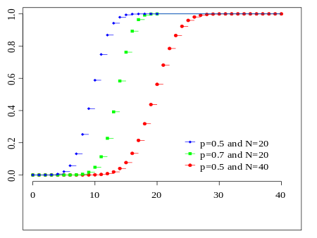
Parameters	n ∈ N0 — number of trials, p ∈ [0,1] — success probability in each trial
Support	$k ∈ { 0, …, n }$ — number of successes
pmf	$\textstyle {n \choose k}\, p^k (1-p)^{n-k}$
CDF	$\textstyle I_{1-p}(n - k, 1 + k)$
Mean	$np$
Median	$\lfloor np \rfloor or \lceil np \rceil$
Mode	$\lfloor (n + 1)p \rfloor or \lceil (n + 1)p \rceil - 1$
Variance	$np(1 - p)$
Skewness	$\frac{1-2p}{\sqrt{np(1-p)}}$
Ex. kurtosis	$\frac{1-6p(1-p)}{np(1-p)}$
Entropy	$\frac12 \log_2 \big( 2\pi e\, np(1-p) \big) + O \left( \frac{1}{n} \right)$ in shannons. For nats, use the natural log in the log.
MGF	$(1-p + pe^t)^n \!$
CF	$(1-p + pe^{it})^n \!$
PGF	$G(z) = \left[(1-p) + pz\right]^n.$
Fisher information	$g_n(p) = \frac{n}{p(1-p)}$ (for fixed n)

Poisson distribution 泊松分布 @

Story @

There are rare events (low probability events) that occur many different ways (high possibilities of occurences) at an average rate of λ occurrences per unit space or time. The number of events that occur in that unit of space or time is X.

Example A certain busy intersection （十字路口）has an average of 2 accidents per month. Since an accident is a low probability event that can happen many different ways, it is reasonable to model the number of accidents in a month at that intersection as Pois(2). Then the number of accidents that happen in two months at that intersection is distributed Pois(4).

速率是 λ, 在时间 n 内发生的次数用 X 来表示，那么 X ~ Poi(λ)

Poission 和泰勒级数是相关的。

Poisson distribution (/ˈpwɑːsɒn/), named after French mathematician Siméon Denis Poisson, is a discrete probability distribution that expresses the probability of a given number of events occurring in a fixed interval of time and/or space if these events occur with a known average rate and independently of the time since the last event. The Poisson distribution can also be used for the number of events in other specified intervals such as distance, area or volume.

A discrete random variable X is said to have a Poisson distribution with parameter λ > 0, if, for k = 0, 1, 2, …, the probability mass function of X is given by:

\[\!f(k; \lambda)= \Pr(X = k)= \frac{\lambda^k e^{-\lambda}}{k!},\]

The positive real number λ is equal to the expected value of X and also to its variance

\[\lambda=\operatorname{E}(X)=\operatorname{Var}(X).\]

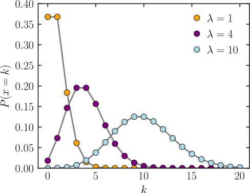
pmf: The horizontal axis is the index k, the number of occurrences. λ is the expected value. The function is defined only at integer values of k. The connecting lines are only guides for the eye.

CDF: The horizontal axis is the index k, the number of occurrences. The CDF is discontinuous at the integers of k and flat everywhere else because a variable that is Poisson distributed takes on only integer values.

Parameters	$λ > 0 (real)$
Support	$k ∈ ℤ*$
pmf	$\frac{\lambda^k e^{-\lambda}}{k!}$
CDF	$\frac{\Gamma(\lfloor k+1\rfloor, \lambda)}{\lfloor k\rfloor !}$, or
	$e^{-\lambda} \sum_{i=0}^{\lfloor k\rfloor} \frac{\lambda^i}{i!}$, or
	$Q(\lfloor k+1\rfloor,\lambda)$ (for $k\ge 0$, where
	$\Gamma(x, y)$ is the incomplete gamma function, $\lfloor k\rfloor$
	is the floor function, and Q is the regularized gamma function)
Mean	$\lambda$
Median	$\approx\lfloor\lambda+1/3-0.02/\lambda\rfloor$
Mode	$\lceil\lambda\rceil - 1, \lfloor\lambda\rfloor$
Variance	$\lambda$
Skewness	$\lambda^{-1/2}$
Ex. kurtosis	$\lambda^{-1}$
Entropy	$\lambda[1 - \log(\lambda)] + e^{-\lambda}\sum_{k=0}^\infty \frac{\lambda^k\log(k!)}{k!} (for large \lambda)$
	$\frac{1}{2}\log(2 \pi e \lambda) - \frac{1}{12 \lambda} - \frac{1}{24 \lambda^2} - \qquad \frac{19}{360 \lambda^3} + O\left(\frac{1}{\lambda^4}\right)$
MGF	$\exp(\lambda (e^{t} - 1))$
CF	$\exp(\lambda (e^{it} - 1))$
PGF	$\exp(\lambda(z - 1))$
Fisher information	$\lambda^{-1}$

Compound Poisson distribution @

In probability theory, a compound Poisson distribution is the probability distribution of the sum of a number of independent identically-distributed random variables, where the number of terms to be added is itself a Poisson-distributed variable. In the simplest cases, the result can be either a continuous or a discrete distribution.

Definition @

Suppose that

\[N\sim\operatorname{Poisson}(\lambda),\]

i.e., N is a random variable whose distribution is a Poisson distribution with expected value λ, and that

\[X_1, X_2, X_3, \dots\]

are identically distributed random variables that are mutually independent and also independent of N. Then the probability distribution of the sum of N i.i.d. random variables conditioned on the number of these variables (N):

\[Y \mid N=\sum_{n=1}^N X_n\]

has a well-defined distribution. In the case N = 0, then the value of Y is 0, so that then Y | N = 0 has a degenerate distribution.

The compound Poisson distribution is obtained by marginalising the joint distribution of (Y,N) over N, where this joint distribution is obtained by combining the conditional distribution Y | N with the marginal distribution of N.

Properties

Mean and variance of the compound distribution derive in a simple way from law of total expectation and the law of total variance. Thus

TODO: Compound Poisson distribution - Wikipedia, the free encyclopedia

Law of total expectation @

The proposition in probability theory known as the law of total expectation, the law of iterated expectations, the tower rule, the smoothing theorem, and Adam’s Law among other names, states that if X is an integrable random variable (i.e., a random variable satisfying E( | X | ) < ∞) and Y is any random variable, not necessarily integrable, on the same probability space, then

\[\operatorname{E} (X) = \operatorname{E} ( \operatorname{E} ( X \mid Y)),\]

i.e., the expected value of the conditional expected value of X given Y is the same as the expected value of X.

The conditional expected value E( X | Y ) is a random variable in its own right, whose value depends on the value of Y. Notice that the conditional expected value of X given the event Y = y is a function of y. If we write E( X | Y = y) = g(y) then the random variable E( X | Y ) is just g(Y).

One special case states that if $A_1, A_2, \ldots, A_n$ is a partition of the whole outcome space, i.e. these events are mutually exclusive and exhaustive, then

\[\operatorname{E} (X) = \sum_{i=1}^{n}{\operatorname{E}(X \mid A_i) \operatorname{P}(A_i)}.\]

TODO: Law of total expectation - Wikipedia, the free encyclopedia

Law of total variance @

In probability theory, the law of total variance or variance decomposition formula, also known as Eve’s law, states that if X and Y are random variables on the same probability space, and the variance of Y is finite, then

\[\operatorname{Var}[Y]=\operatorname{E}(\operatorname{Var}[Y\mid X])+\operatorname{Var}(\operatorname{E}[Y\mid X]).\,\]

不仅概率可以分块加，variance 也可以。

TODO: Law of total variance - Wikipedia, the free encyclopedia

Poisson approximation @

the Poisson distribution with parameter λ = np can be used as an approximation to B(n, p) of the binomial distribution if n is sufficiently large and p is sufficiently small.

Limiting distributions

Poisson limit theorem: As n approaches ∞ and p approaches 0, then the Binomial(n, p) distribution approaches the Poisson distribution with expected value λ
de Moivre–Laplace theorem: As n approaches ∞ while p remains fixed, the distribution of \[\frac{X-np}{\sqrt{np(1-p)}}\]

approaches the normal distribution with expected value 0 and variance 1. This result is sometimes loosely stated by saying that the distribution of X is asymptotically normal with expected value np and variance np(1 − p). This result is a specific case of the central limit theorem.

这个看成 normalize 就可以了。X_normalized = (X - mean)/variance

Poisson limit theorem @

The law of rare events or Poisson limit theorem gives a Poisson approximation to the binomial distribution, under certain conditions. The theorem was named after Siméon Denis Poisson (1781–1840).

If $n \rightarrow \infty, p \rightarrow 0, \text{such that } np \rightarrow \lambda$, then

\[\frac{n!}{(n-k)!k!} p^k (1-p)^{n-k} \rightarrow e^{-\lambda}\frac{\lambda^k}{k!}.\]

Negative binomial distribution @

Different texts adopt slightly different definitions for the negative binomial distribution. They can be distinguished by whether the support starts at k = 0 or at k = r, whether p denotes the probability of a success or of a failure, and whether r represents success or failure, so it is crucial to identify the specific parametrization used in any given text.

Notation	$\mathrm{NB}(r,\,p)$
Parameters	r > 0 — number of failures until the experiment is stopped, p ∈ (0,1) — success probability in each experiment (real)
Support	k ∈ { 0, 1, 2, 3, … } — number of successes
pmf	${k+r-1 \choose k}\cdot (1-p)^r p^k,\!$ involving a binomial coefficient³
CDF	$1-I_p(k+1,\,r)$, the regularized incomplete beta function
Mean	$\frac{pr}{1-p}$
Mode	$\begin{cases}\big\lfloor\frac{p(r-1)}{1-p}\big\rfloor & \text{if}\ r>1 \\ 0 & \text{if}\ r\leq 1\end{cases}$
Variance	$\frac{pr}{(1-p)^2}$
Skewness	$\frac{1+p}{\sqrt{pr}}$

Suppose there is a sequence of independent Bernoulli trials. Thus, each trial has two potential outcomes called “success” and “failure”. In each trial the probability of success is p and of failure is (1 − p). We are observing this sequence until a predefined number r of failures has occurred. Then the random number of successes we have seen, X, will have the negative binomial (or Pascal) distribution:

\[X\sim\operatorname{NB}(r; p)\]

Geometric distribution @

Story @

X is the number of “failures” that we will achieve before we achieve our first success. Our successes have probability p.

Example If each pokeball we throw has probability 1/10 to catch Mew, the number of failed pokeballs will be distributed Geom( 1/10 ).

These two different geometric distributions should not be confused with each other. Often, the name shifted geometric distribution is adopted for the former one (distribution of the number X); however, to avoid ambiguity, it is considered wise to indicate which is intended, by mentioning the support explicitly.

It’s the probability that the first occurrence of success requires k number of independent trials, each with success probability p. If the probability of success on each trial is p, then the probability that the kth trial (out of k trials) is the first success is

\[\Pr(X = k) = (1-p)^{k-1}\,p\,\]

for k = 1, 2, 3, ….

The above form of geometric distribution is used for modeling the number of trials up to and including the first success. By contrast, the following form of the geometric distribution is used for modeling the number of failures until the first success:

\[\Pr(Y=k) = (1 - p)^k\,p\,\]

for k = 0, 1, 2, 3, ….

pmf & CDF

Parameters	0< p $\leq$ 1 success probability (real)	0< p $\leq$ 1 success probability (real)
Support	k trials where $k \in \{1,2,3,\dots\}\!$	k failures where $k \in \{0,1,2,3,\dots\}\!$
pmf	$(1 - p)^{k-1}\,p\!$	$(1 - p)^{k}\,p\!$
CDF	$1-(1 - p)^k\!$	$1-(1 - p)^{k+1}\!$
Mean	$\frac{1}{p}\!$	$\frac{1-p}{p}\!$
Median	$\left\lceil \frac{-1}{\log_2(1-p)} \right\rceil\!$	$\left\lceil \frac{-1}{\log_2(1-p)} \right\rceil\! - 1$
Mode	1	0
Variance	$\frac{1-p}{p^2}\!$	$\frac{1-p}{p^2}\!$
Skewness	$\frac{2-p}{\sqrt{1-p}}\!$	$\frac{2-p}{\sqrt{1-p}}\!$
Excess kurtosis	$6+\frac{p^2}{1-p}\!$	$6+\frac{p^2}{1-p}\!$
Entropy	$\tfrac{-(1-p)\log_2 (1-p) - p \log_2 p}{p}\!$	$\tfrac{-(1-p)\log_2 (1-p) - p \log_2 p}{p}\!$
mgf	$\frac{pe^t}{1-(1-p) e^t}\!, for t<-\ln(1-p)\!$	$\frac{p}{1-(1-p)e^t}\!$
Characteristic function	$\frac{pe^{it}}{1-(1-p)\,e^{it}}\!$	$\frac{p}{1-(1-p)\,e^{it}}\!$

The expected value of a geometrically distributed random variable X is 1/p and the variance is (1 − p)/p2:

\[\mathrm{E}(X) = \frac{1}{p}, \qquad\mathrm{var}(X) = \frac{1-p}{p^2}.\]

Hypergeometric distribution @

A random variable X follows the hypergeometric distribution if its probability mass function (pmf) is given by

\[ P(X = k) = \frac{\binom{K}{k} \binom{N - K}{n-k}}{\binom{N}{n}}, \]

where

N is the population size,
K is the number of success states in the population,
n is the number of draws,
k is the number of observed successes,
$\textstyle {a \choose b}$ is a binomial coefficient.

Continuous Uniform distribution @

In probability theory and statistics, the continuous uniform distribution or rectangular distribution is a family of symmetric probability distributions such that for each member of the family, all intervals of the same length on the distribution’s support are equally probable. The support is defined by the two parameters, a and b, which are its minimum and maximum values. The distribution is often abbreviated U(a,b). It is the maximum entropy probability distribution for a random variate X under no constraint other than that it is contained in the distribution’s support.

Notation	$\mathcal{U}(a, b)$ or $\mathrm{unif}(a,b)$
Parameters	$-\infty < a < b < \infty \,$
Support	$x \in [a,b]$
PDF	$\begin{cases} \frac{1}{b - a} & \text{for } x \in [a,b] \\ 0 & \text{otherwise} \end{cases}$
CDF	$\begin{cases} 0 & \text{for } x < a \\ \frac{x-a}{b-a} & \text{for } x \in [a,b) \\ 1 & \text{for } x \ge b \end{cases}$
Mean	$\tfrac{1}{2}(a+b)$
Median	$\tfrac{1}{2}(a+b)$
Mode	any value in (a,b)
Variance	$\tfrac{1}{12}(b-a)^2$
Skewness	0
Ex. kurtosis	$-\tfrac{6}{5}$
Entropy	$\log(b-a) \,$
MGF	$\begin{cases} \frac{\mathrm{e}^{tb}-\mathrm{e}^{ta}}{t(b-a)} &\text{for } t \neq 0 \\ 1 &\text{for } t = 0 \end{cases}$
CF	$\frac{\mathrm{e}^{itb}-\mathrm{e}^{ita}}{it(b-a)}$

Error function @

Plot of the error function

(erf: a sigmoid)

In mathematics, the error function (also called the Gauss error function) is a special function (non-elementary) of sigmoid shape that occurs in probability, statistics, and partial differential equations describing diffusion. It is defined as:

\[\operatorname{erf}(x) = \frac{2}{\sqrt\pi}\int_0^x e^{-t^2}\,\mathrm dt.\]

The complementary error function, denoted erfc, is defined as

\[\begin{align} \operatorname{erfc}(x) & = 1-\operatorname{erf}(x) \\ & = \frac{2}{\sqrt\pi} \int_x^{\infty} e^{-t^2}\,\mathrm dt \\ & = e^{-x^2} \operatorname{erfcx}(x), \end{align}\]

which also defines erfcx, the scaled complementary error function (which can be used instead of erfc to avoid arithmetic underflow). Another form of $\operatorname{erfc}(x)$ is known as Craig’s formula:

\[\begin{align} \operatorname{erfc}(x) & = \frac{2}{\pi} \int_0^{\pi/2} \exp \left( - \frac{x^2}{\sin^2 \theta} \right) d\theta. \end{align}\]

The error function is related to the cumulative distribution , the integral of the standard normal distribution, by

\[\Phi (x) = \frac{1}{2}+ \frac{1}{2} \operatorname{erf} \left(x/ \sqrt{2}\right) = \frac{1}{2} \operatorname{erfc} \left(-x/ \sqrt{2}\right).\]

Q-function @

A plot of the Q-function.

In statistics, the Q-function is the tail probability of the standard normal distribution (x). In other words, Q(x) is the probability that a normal (Gaussian) random variable will obtain a value larger than x standard deviations above the mean.

If the underlying random variable is y, then the proper argument to the tail probability is derived as:

\[x=\frac{y - \mu}{\sigma}\]

which expresses the number of standard deviations away from the mean.

Because of its relation to the cumulative distribution function of the normal distribution, the Q-function can also be expressed in terms of the error function, which is an important function in applied mathematics and physics.

Formally, the Q-function is defined as

\[Q(x) = \frac{1}{\sqrt{2\pi}} \int_x^\infty \exp\left(-\frac{u^2}{2}\right) \, du.\]

Thus,

\[Q(x) = 1 - Q(-x) = 1 - \Phi(x)\,\!,\]

where $\Phi(x)$ is the cumulative distribution function of the normal Gaussian distribution.

Normal distribution @

(also, Z distribution)

The probability density of the normal distribution is:

\[f(x \; | \; \mu, \sigma^2) = \frac{1}{\sigma\sqrt{2\pi} } \; e^{ -\frac{(x-\mu)^2}{2\sigma^2} }\]

Where:

$\mu$ is mean or expectation of the distribution (and also its median and mode).
$\sigma$ is standard deviation
$\sigma^2$ is variance

pdf & CDF

Notation	$\mathcal{N}(\mu,\,\sigma^2)$
Parameters	μ ∈ R — mean (location), σ2 > 0 — variance (squared scale)
Support	$x ∈ R$
PDF	$\frac{1}{\sigma\sqrt{2\pi}}\, e^{-\frac{(x - \mu)^2}{2 \sigma^2}}$
CDF	$\frac12\left[1 + \operatorname{erf}\left( \frac{x-\mu}{\sigma\sqrt{2}}\right)\right]$
Quantile	$\mu+\sigma\sqrt{2}\,\operatorname{erf}^{-1}(2F-1)$
Mean	μ
Median	μ
Mode	μ
Variance	$\sigma^2\,$
Skewness	0
Ex. kurtosis	0
Entropy	$\tfrac12 \ln(2\pi\,e\,\sigma^2)$
MGF	$\exp\{ \mu t + \frac{1}{2}\sigma^2t^2 \}$
CF	$\exp \{ i\mu t - \frac{1}{2}\sigma^2 t^2 \}$
Fisher information	$\begin{pmatrix}1/\sigma^2&0\\0&1/(2\sigma^4)\end{pmatrix}$

Standard normal distribution

\[\phi(x) = \frac{e^{- \frac{\scriptscriptstyle 1}{\scriptscriptstyle 2} x^2}}{\sqrt{2\pi}}\,\]

Standard deviation and tolerance intervals @

For the normal distribution, the values less than one standard deviation away from the mean account for 68.27% of the set; while two standard deviations from the mean account for 95.45%; and three standard deviations account for 99.73%.

the probability that a normal deviate lies in the range μ − nσ and μ + nσ is given by

\[F(\mu+n\sigma) - F(\mu-n\sigma) = \Phi(n)-\Phi(-n) = \mathrm{erf}\left(\frac{n}{\sqrt{2}}\right),\]

Cumulative distribution function @

The cumulative distribution function (CDF) of the standard normal distribution, usually denoted with the capital Greek letter (phi), is the integral

\[\Phi(x)\; = \;\frac{1}{\sqrt{2\pi}} \int_{-\infty}^x e^{-t^2/2} \, dt\]

In statistics one often uses the related error function, or erf(x), defined as the probability of a random variable with normal distribution of mean 0 and variance 1/2 falling in the range [-x, x]; that is

\[\operatorname{erf}(x)\; =\; \frac{1}{\sqrt{\pi}} \int_{-x}^x e^{-t^2} \, dt\]

These integrals cannot be expressed in terms of elementary functions, and are often said to be special functions. However, many numerical approximations are known; see below.

正太分布的 CDF 和 erf 很像。满足如下关系。

The two functions are closely related, namely

\[\Phi(x)\; =\; \frac12\left[1 + \operatorname{erf}\left(\frac{x}{\sqrt{2}}\right)\right]\]

For a generic normal distribution f with mean μ and deviation σ, the cumulative distribution function is

\[F(x)\;=\;\Phi\left(\frac{x-\mu}{\sigma}\right)\;=\; \frac12\left[1 + \operatorname{erf}\left(\frac{x-\mu}{\sigma\sqrt{2}}\right)\right]\]

Standard score @

Z-分数，所以正太分布也叫 z 分布。标准分布，在考试测验评分里常用。

Standard scores are also called z-values, z-scores, normal scores, and standardized variables; the use of “Z” is because the normal distribution is also known as the “Z distribution”. They are most frequently used to compare a sample to a standard normal deviate, though they can be defined without assumptions of normality.

Compares the various grading methods in a normal distribution. Includes: Standard deviations, cumulative percentages, percentile equivalents, Z-scores, T-scores, standard nine, percent in stanine

The standard score of a raw score x is

\[z = {x- \mu \over \sigma}\]

In mathematical statistics, a random variable X is standardized by subtracting its expected value $\operatorname{E}[X]$ and dividing the difference by its standard deviation $\sigma(X) = \sqrt{\operatorname{Var}(X)}$:

\[Z = {X - \operatorname{E}[X] \over \sigma(X)}\]

Stanine

标准九。

Stanine (STAndard NINE) is a method of scaling test scores on a nine-point standard scale with a mean of five and a standard deviation of two.

Calculating Stanines

Result Ranking	4%	7%	12%	17%	20%	17%	12%	7%	4%
Stanine	1	2	3	4	5	6	7	8	9
Standard score	below -1.75	-1.75 to -1.25	-1.25 to -.75	-.75 to -.25	-.25 to +.25	+.25 to +.75	+.75 to +1.25	+1.25 to +1.75	above +1.75
Wechsler scale score	below 74	74 to 81	81 to 89	89 to 96	96 to 104	104 to 111	111 to 119	119 to 126	above 126

Today stanines are mostly used in educational assessment.

t-statistic @

notional, ['noʊʃən(ə)l] adj.猜测的；估计的；理论上的；想象的

用于假设检验。

In statistics, the t-statistic is a ratio of the departure of an estimated parameter from its notional value and its standard error. It is used in hypothesis testing, for example in the Student’s t-test, in the augmented Dickey–Fuller test, and in bootstrapping.

Let $\scriptstyle\hat\beta$ be an estimator of parameter β in some statistical model. Then a t-statistic for this parameter is any quantity of the form

\[t_{\hat{\beta}} = \frac{\hat\beta - \beta_0}{\mathrm{s.e.}(\hat\beta)}\]

where β0 is a non-random, known constant, and $\scriptstyle s.e.(\hat\beta)$ is the standard error of the estimator $\scriptstyle\hat\beta$. By default, statistical packages report t-statistic with β0 = 0 (these t-statistics are used to test the significance of corresponding regressor). However, when t-statistic is needed to test the hypothesis of the form H0: β = β0, then a non-zero β0 may be used.

If $\scriptstyle\hat\beta$ is an ordinary least squares estimator in the classical linear regression model (that is, with normally distributed and homoskedastic error terms), and if the true value of parameter β is equal to β0, then the sampling distribution of the t-statistic is the Student’s t-distribution with (n − k) degrees of freedom, where n is the number of observations, and k is the number of regressors (including the intercept).

In the majority of models the estimator is consistent for β and distributed asymptotically normally. If the true value of parameter β is equal to β0 and the quantity $\scriptstyle s.e.(\hat\beta)$ correctly estimates the asymptotic variance of this estimator, then the t-statistic will have asymptotically the standard normal distribution.

In some models the distribution of t-statistic is different from normal, even asymptotically. For example, when a time series with unit root is regressed in the augmented Dickey–Fuller test, the test t-statistic will asymptotically have one of the Dickey–Fuller distributions (depending on the test setting).

Exponential distribution @

Story @

You’re sitting on an open meadow right before the break of dawn, wishing that airplanes in the night sky were shooting stars, because you could really use a wish right now. You know that shooting stars come on average every 15 minutes, but a shooting star is not “due” to come just because you’ve waited so long. Your waiting time is memoryless; the additional time until the next shooting star comes does not depend on how long you’ve waited already.

Example The waiting time until the next shooting star is distributed Expo(4) hours. Here λ = 4 is the rate parameter, since shooting stars arrive at a rate of 1 per 1/4 hour on average. The expected time until the next shooting star is 1/λ = 1/4 hour.

Expo(λ)，λ 是单位时间流星的个数，1/λ 是你等到下一个流星需要等待的时间（的期望）。

The exponential distribution (a.k.a. negative exponential distribution) is the probability distribution that describes the time between events in a Poisson process, i.e. a process in which events occur continuously and independently at a constant average rate. It is a particular case of the gamma distribution. It is the continuous analogue of the geometric distribution, and it has the key property of being memoryless. In addition to being used for the analysis of Poisson processes, it is found in various other contexts.

The exponential distribution is not the same as the class of exponential families of distributions, which is a large class of probability distributions that includes the exponential distribution as one of its members, but also includes the normal distribution, binomial distribution, gamma distribution, Poisson, and many others.

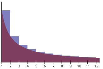
pdf & CDF

The probability density function (pdf) of an exponential distribution is

\[ f(x;\lambda) = \begin{cases} \lambda e^{-\lambda x} & x \ge 0, \\ 0 & x < 0. \end{cases} \]

Alternatively, this can be defined using the right-continuous Heaviside step function, H(x) where H(0)=1:

\[ f(x;\lambda) = \mathrm \lambda e^{-\lambda x} H(x) \]

Heaviside step function - Wikipedia, the free encyclopedia @

The Heaviside ([ˈhevisaid]) step function, or the unit step function, usually denoted by θ (but sometimes u or 𝟙), is a discontinuous function whose value is zero for negative argument and one for positive argument. It is an example of the general class of step functions, all of which can be represented as linear combinations of translations of this one.

The Heaviside step function, using the half-maximum convention

The simplest definition of the Heaviside function is as the derivative of the ramp function:

\[H(x) := \frac{d}{dx} \max \{ x, 0 \}\]

The Heaviside function can also be defined as the integral of the Dirac delta function: H′ = δ. This is sometimes written as

\[H(x) := \int_{-\infty}^x { \delta(s)} \, \mathrm{d}s\]

Parameters	λ > 0 rate, or inverse scale
Support	$x ∈ [0, ∞)$
PDF	$λ e−λx$
CDF	$1 − e−λx$
Quantile	$-ln(1-F)/λ$
Mean	$λ−1 (=β)$
Median	$λ−1 ln(2)$
Mode	0
Variance	$λ−2 (=β2)$
Skewness	2
Ex. kurtosis	6
Entropy	$log(e/λ)$
MGF	$\frac{\lambda}{\lambda-t}, \text{ for } t < \lambda$
CF	$\frac{\lambda}{\lambda-it}$
Fisher information	$^{-2} $

Gamma distribution @

Story @

You sit waiting for shooting stars, where the waiting time for a star is distributed Expo(λ). You want to see n shooting stars before you go home. The total waiting time for the nth shooting star is Gamma(n,λ).

Example You are at a bank, and there are 3 people ahead of you. The serving time for each person is Exponential with mean 2 minutes. Only one person at a time can be served. The distribution of your waiting time until it’s your turn to be served is Gamma(3, 1/2 ).

还是等流星，Expo(λ)，意思是单位时间可以有 λ 个流星，1/λ 的时间预期可以等到一个。你想看到 n 个流星再回家，那么你的等待时间满足 Gamma(n,λ) 分布。排队也是一样的。

（但是感觉这两种不太一样，因为流星之间是无关的，而排队的人是有序的。）

In probability theory and statistics, the gamma distribution is a two-parameter family of continuous probability distributions. The common exponential distribution and chi-squared distribution are special cases of the gamma distribution. There are three different parametrizations in common use:

With a shape parameter k and a scale parameter θ.
With a shape parameter α = k and an inverse scale parameter β = 1/θ, called a rate parameter.
With a shape parameter k and a mean parameter μ = k/β.

pdf & CDF

Parameters	k > 0 shape, θ > 0 scale	α > 0 shape, β > 0 rate
Support	$\scriptstyle x \;\in\; (0,\, \infty)$	$\scriptstyle x \;\in\; (0,\, \infty)$
pdf	$\frac{1}{\Gamma(k) \theta^k} x^{k \,-\, 1} e^{-\frac{x}{\theta}}$	$\frac{\beta^\alpha}{\Gamma(\alpha)} x^{\alpha \,-\, 1} e^{- \beta x }$
CDF	$\frac{1}{\Gamma(k)} \gamma\left(k,\, \frac{x}{\theta}\right)$	$\frac{1}{\Gamma(\alpha)} \gamma(\alpha,\, \beta x)$
Mean	$\scriptstyle \mathbf{E}[ X] = k \theta$	$\scriptstyle\mathbf{E}[ X] = \frac{\alpha}{\beta}$
	$\scriptstyle \mathbf{E}[\ln X] = \psi(k) +\ln(\theta)$	$\scriptstyle \mathbf{E}[\ln X] = \psi(\alpha) -\ln(\beta)$
Median	No simple closed form	No simple closed form
Mode	$\scriptstyle (k \,-\, 1)\theta \text{ for } k \;{\geq}\; 1$	$\scriptstyle \frac{\alpha \,-\, 1}{\beta} \text{ for } \alpha \;{\geq}\; 1$
Variance	$\scriptstyle\operatorname{Var}[ X] = k \theta^2$	$\scriptstyle \operatorname{Var}[ X] = \frac{\alpha}{\beta^2}$
	$\scriptstyle\operatorname{Var}[\ln X] = \psi_1(k)$	$\scriptstyle\operatorname{Var}[\ln X] = \psi_1(\alpha)$
Skewness	$\scriptstyle \frac{2}{\sqrt{k}}$	$\scriptstyle \frac{2}{\sqrt{\alpha}}$
Excess kurtosis	$\scriptstyle \frac{6}{k}$	$\scriptstyle \frac{6}{\alpha}$

Beta distribution @

In probability theory and statistics, the beta distribution is a family of continuous probability distributions defined on the interval [0, 1] parametrized by two positive shape parameters, denoted by α and β, that appear as exponents of the random variable and control the shape of the distribution.

The beta distribution has been applied to model the behavior of random variables limited to intervals of finite length in a wide variety of disciplines. For example, it has been used as a statistical description of allele frequencies in population genetics; time allocation in project management / control systems; sunshine data; variability of soil properties; proportions of the minerals in rocks in stratigraphy; and heterogeneity in the probability of HIV transmission.

In Bayesian inference, the beta distribution is the conjugate prior probability distribution for the Bernoulli, binomial, negative binomial and geometric distributions. For example, the beta distribution can be used in Bayesian analysis to describe initial knowledge concerning probability of success such as the probability that a space vehicle will successfully complete a specified mission. The beta distribution is a suitable model for the random behavior of percentages and proportions.

The usual formulation of the beta distribution is also known as the beta distribution of the first kind, whereas beta distribution of the second kind is an alternative name for the beta prime distribution.

pdf & CDF

Notation	Beta(α, β)
Parameters	α > 0 shape (real), β > 0 shape (real)
Support	$x \in (0, 1)\!$
PDF	$\frac{x^{\alpha-1}(1-x)^{\beta-1}} {\operatorname{Beta}(\alpha,\beta)}\!$ where $\operatorname{Beta}(\alpha,\beta) = \frac{\Gamma(\alpha)\Gamma(\beta)}{\Gamma(\alpha + \beta)}$
CDF	$I_x(\alpha,\beta)\!$
Mean	$\operatorname{E}[X] = \frac{\alpha}{\alpha+\beta}\!$, $\operatorname{E}[\ln X] = \psi(\alpha) - \psi(\alpha + \beta)\!$
Median	$\begin{matrix}I_{\frac{1}{2}}^{[-1]}(\alpha,\beta)\text{ (in general) }\\[0.5em] \approx \frac{ \alpha - \tfrac{1}{3} }{ \alpha + \beta - \tfrac{2}{3} }\text{ for }\alpha, \beta >1\end{matrix}$
Mode	$\frac{\alpha-1}{\alpha+\beta-2}\!$ for α, β >1
Variance	$\operatorname{var}[X] = \frac{\alpha\beta}{(\alpha+\beta)^2(\alpha+\beta+1)}\!$, $\operatorname{var}[\ln X] = \psi_1(\alpha) - \psi_1(\alpha + \beta)\!$
Skewness	$\frac{2\,(\beta-\alpha)\sqrt{\alpha+\beta+1}}{(\alpha+\beta+2)\sqrt{\alpha\beta}}$
Ex. kurtosis	$\frac{6[(\alpha - \beta)^2 (\alpha +\beta + 1) - \alpha \beta (\alpha + \beta + 2)]}{\alpha \beta (\alpha + \beta + 2) (\alpha + \beta + 3)}$
Entropy	$\begin{matrix}\ln\operatorname{Beta}(\alpha,\beta)-(\alpha-1)\psi(\alpha)-(\beta-1)\psi(\beta)\\[0.5em] +(\alpha+\beta-2)\psi(\alpha+\beta)\end{matrix}$
MGF	$1 +\sum_{k=1}^{\infty} \left( \prod_{r=0}^{k-1} \frac{\alpha+r}{\alpha+\beta+r} \right) \frac{t^k}{k!}$
CF	${}_1F_1(\alpha; \alpha+\beta; i\,t)\!$
Fisher information	$\begin{matrix}\\ \operatorname{var}[\ln X] &\operatorname{cov}[\ln X, \ln(1-X)] \\ \operatorname{cov}[\ln X, \ln(1-X)] & \operatorname{var}[\ln (1-X)]\end{matrix}$

Tolerance interval @

A tolerance interval is a statistical interval within which, with some confidence level, a specified proportion of a sampled population falls.

“More speciﬁcally, a 100×p%/100×(1−α) tolerance interval provides limits within which at least a certain proportion (p) of the population falls with a given level of confidence (1−α).”

“A (p, 1−α) tolerance interval (TI) based on a sample is constructed so that it would include at least a proportion p of the sampled population with confidence 1−α; such a TI is usually referred to as p-content −(1−α) coverage TI.”

“A (p, 1−α) upper tolerance limit (TL) is simply an 1−αupper confidence limit for the 100 p percentile of the population.”

A tolerance interval can be seen as a statistical version of a probability interval. “In the parameters-known case, a 95% tolerance interval and a 95% prediction interval are the same.” If we knew a population’s exact parameters, we would be able to compute a range within which a certain proportion of the population falls. For example, if we know a population is normally distributed with mean and standard deviation , then the interval 1.96includes 95% of the population (1.96 is the z-score for 95% coverage of a normally distributed population).

Gamma function @

In mathematics, the gamma function (represented by the capital Greek letter Γ) is an extension of the factorial function, with its argument shifted down by 1, to real and complex numbers. That is, if n is a positive integer:

\[\Gamma(n) = (n-1)!.\]

The gamma function is defined for all complex numbers except the non-positive integers. For complex numbers with a positive real part, it is defined via a convergent improper integral:

\[\Gamma(t) = \int_0^\infty x^{t-1} e^{-x}\,dx.\]

This integral function is extended by analytic continuation to all complex numbers except the non-positive integers (where the function has simple poles), yielding the meromorphic ([,merə'mɔːfɪk], 亚纯的) function we call the gamma function. In fact the gamma function corresponds to the Mellin transform of the negative exponential function:

\[\Gamma(t) = \{ \mathcal M e^{-x} \} (t).\]

The gamma function is meromorphic in the whole complex plane.

The gamma function is a component in various probability-distribution functions, and as such it is applicable in the fields of probability and statistics, as well as combinatorics.

It is easy graphically to interpolate the factorial function to non-integer values, but is there a formula that describes the resulting curve?

Properties

$\Gamma(t+1)=t \Gamma(t)\,$, Γ(t) = Γ(t + 1)/t, $\Gamma(t)=\frac{\Gamma(t+n)}{t(t+1)\cdots(t+n-1)},$
$\Gamma(n) = 1 \cdot 2 \cdot 3 \cdots (n-1) = (n-1)!\,$
$\Gamma\left(\tfrac{1}{2}\right)=\sqrt{\pi},$
$\Gamma\left(\tfrac{1}{2}+n\right) = {(2n)! \over 4^n n!} \sqrt{\pi} = \frac{(2n-1)!!}{2^n} \sqrt{\pi} = \sqrt{\pi} \left[ {n-\frac{1}{2}\choose n} n! \right]$
$\Gamma\left(\tfrac{1}{2}-n\right) = {(-4)^n n! \over (2n)!} \sqrt{\pi} = \frac{(-2)^n}{(2n-1)!!} \sqrt{\pi} = \frac{\sqrt{\pi}}{{-\frac{1}{2} \choose n} n!}$

Pi function

An alternative notation which was originally introduced by Gauss and which was sometimes used is the pi function, which in terms of the gamma function is

\[\Pi(z) = \Gamma(z+1) = z \Gamma(z) = \int_0^\infty e^{-t} t^z\, dt,\]

For Re(x) > 0 the nth derivative of the gamma function is:

\[\frac{{\rm d}^n}{{\rm d}x^n}\,\Gamma(x) = \int_0^\infty t^{x-1} e^{-t} (\ln t)^{n} dt.\]

Stirling’s formula

Asymptotically (逐渐地) as t → ∞, the magnitude of the gamma function is given by Stirling’s formula

\[\Gamma(t+1)\sim\sqrt{2\pi t}\left(\frac{t}{e}\right)^{t},\]

where the symbol ~ means that the quotient of both sides converges to 1.

Euler’s reflection formula

\[\Gamma(1-z) \Gamma(z) = {\pi \over \sin{(\pi z)}}, \qquad z \not\in \mathbf Z\]

Duplication formula

\[\Gamma(z) \Gamma\left(z + \tfrac{1}{2}\right) = 2^{1-2z} \; \sqrt{\pi} \; \Gamma(2z).\]

The duplication formula is a special case of the multiplication theorem

\[\prod_{k=0}^{m-1}\Gamma\left(z + \frac{k}{m}\right) = (2 \pi)^{\frac{m-1}{2}} \; m^{\frac{1}{2} - mz} \; \Gamma(mz).\]

Meromorphic function

In the mathematical field of complex analysis, a meromorphic function on an open subset D of the complex plane is a function that is holomorphic on all D except a set of isolated points (the poles of the function), at each of which the function must have a Laurent series. This terminology comes from the Ancient Greek meros (μέρος), meaning part, as opposed to holos (ὅλος), meaning whole.

Mellin transform

In mathematics, the Mellin transform is an integral transform that may be regarded as the multiplicative version of the two-sided Laplace transform. This integral transform is closely connected to the theory of Dirichlet series, and is often used in number theory, mathematical statistics, and the theory of asymptotic expansions; it is closely related to the Laplace transform and the Fourier transform, and the theory of the gamma function and allied special functions.

The Mellin transform of a function f is

\[\left\{\mathcal{M}f\right\}(s) = \varphi(s)=\int_0^{\infty} x^{s-1} f(x)dx.\]

The inverse transform is

\[\left\{\mathcal{M}^{-1}\varphi\right\}(x) = f(x)=\frac{1}{2 \pi i} \int_{c-i \infty}^{c+i \infty} x^{-s} \varphi(s)\, ds.\]

refs and see also

Mellin transform - Wikipedia, the free encyclopedia

TODO: Gamma function - Wikipedia, the free encyclopedia

Digamma function @

这个定义和这个希腊字母也太贴切了……

In mathematics, the digamma function is defined as the logarithmic derivative of the gamma function:

\[\psi(x)=\frac{d}{dx}\ln\Big(\Gamma(x)\Big)=\frac{\Gamma'(x)}{\Gamma(x)}.\]

It is the first of the polygamma functions.

The digamma function is often denoted as ψ0(x), ψ0(x) or $\digamma$ (after the archaic Greek letter Ϝ digamma).

Psi (uppercase Ψ, lowercase ψ; Greek: Ψι Psi)

Relation to harmonic numbers @

The gamma function obeys the equation

\[\Gamma(z+1)=z\Gamma(z).\]

Taking the derivative with respect to z gives:

\[\Gamma'(z+1)=z\Gamma'(z)+\Gamma(z)\]

Dividing by Γ(z+1) or the equivalent zΓ(z) gives:

\[\frac{\Gamma'(z+1)}{\Gamma(z+1)}=\frac{\Gamma'(z)}{\Gamma(z)}+\frac 1z\]

or:

\[\psi(z+1)=\psi(z)+\frac 1z\]

Since the harmonic numbers are defined as

\[H_n=\sum_{k=1}^n\frac 1k\]

the digamma function is related to it by:

\[\psi(n)=H_{n-1}-\gamma\]

where $H_n$ is the n-th harmonic number, and γ is the Euler-Mascheroni constant. For half-integer values, it may be expressed as

\[\psi\left(n+{\frac{1}{2}}\right)=-\gamma-2\ln(2)+\sum_{k=1}^n \frac{2}{2k-1}\]

Euler–Mascheroni constant @

The Euler–Mascheroni constant (also called Euler’s constant) is a mathematical constant recurring in analysis and number theory, usually denoted by the lowercase Greek letter gamma (γ).

The area of the blue region converges to the Euler–Mascheroni constant.

It is defined as the limiting difference between the harmonic series and the natural logarithm:

\[\begin{align} \gamma &= \lim_{n\to\infty}\left(-\ln n + \sum_{k=1}^n \frac1{k}\right)\\ &=\int_1^\infty\left(\frac1{\lfloor x\rfloor}-\frac1{x}\right)\,dx. \end{align}\]

The numerical value of the Euler–Mascheroni constant, to 50 decimal places, is

0.57721566490153286060651209008240243104215933593992….

Regularization

The Digamma function appears in the regularization of divergent integrals

\[\int_{0}^{\infty} \frac{dx}{x+a},\]

this integral can be approximated by a divergent general Harmonic series, but the following value can be attached to the series

\[\sum_{n=0}^{\infty} \frac{1}{n+a}= - \psi (a).\]

Integral representations @

If the real part of x is positive then the digamma function has the following integral representation

\[\psi(x)=\int\limits_0^\infty \left(\frac{e^{-t}}{t}-\frac{e^{-xt}}{1-e^{-t}}\right)dt.\]

Beta function @

In mathematics, the beta function, also called the Euler integral of the first kind, is a special function defined by

\[{\operatorname{Beta}}(x,y) = \int_0^1t^{x-1}(1-t)^{y-1}\,\mathrm{d}t \!\]

for $\textrm{Re}(x), \textrm{Re}(y) > 0.\,$

The beta function was studied by Euler and Legendre and was given its name by Jacques Binet; its symbol Β is a Greek capital β rather than the similar Latin capital B.

其实是两个参数控制了形状。这个形状可能是某个 rv 的概率密度。如果 x = y = 1, 于是变成了 0-1 连续均匀分布。因为对称性，a，b 大于 1 的时候，形状是 bell shape，如果 a 更大，整体越右偏。

properties

symmetric: ${\operatorname{Beta}}(x,y) = {\operatorname{Beta}}(y,x). \!$
relationship between gamma function and beta function: ${\operatorname{Beta}}(x,y)=\dfrac{\Gamma(x)\,\Gamma(y)}{\Gamma(x+y)} \!$

When x and y are positive integers, it follows from the definition of the gamma function $\Gamma$ that:
- ${\operatorname{Beta}}(x,y)=\dfrac{(x-1)!\,(y-1)!}{(x+y-1)!} \!$
- ${\operatorname{Beta}}(x,y) = 2\int_0^{\pi/2}(\sin\theta)^{2x-1}(\cos\theta)^{2y-1}\,\mathrm{d}\theta, \qquad \mathrm{Re}(x)>0,\ \mathrm{Re}(y)>0 \!$
- ${\operatorname{Beta}}(x,y) = \int_0^\infty\dfrac{t^{x-1}}{(1+t)^{x+y}}\,\mathrm{d}t, \qquad \mathrm{Re}(x)>0,\ \mathrm{Re}(y)>0 \!$
- ${\operatorname{Beta}}(x,y) = \sum_{n=0}^\infty \dfrac{{n-y \choose n}} {x+n}, \!$
- ${\operatorname{Beta}}(x,y) = \frac{x+y}{x y} \prod_{n=1}^\infty \left( 1+ \dfrac{x y}{n (x+y+n)}\right)^{-1}, \!$
The Beta function satisfies several interesting identities, including
- ${\operatorname{Beta}}(x,y) = {\operatorname{Beta}}(x, y+1) + {\operatorname{Beta}}(x+1, y) \!$
- ${\operatorname{Beta}}(x+1,y) = {\operatorname{Beta}}(x, y) \cdot \dfrac{x}{x+y} \!$
- ${\operatorname{Beta}}(x,y+1) = {\operatorname{Beta}}(x, y) \cdot \dfrac{y}{x+y} \!$
- ${\operatorname{Beta}}(x,y)\cdot(t \mapsto t_+^{x+y-1}) = (t \to t_+^{x-1}) * (t \to t_+^{y-1}) \qquad x\ge 1, y\ge 1, \!$
- ${\operatorname{Beta}}(x,y) \cdot {\operatorname{Beta}}(x+y,1-y) = \dfrac{\pi}{x \sin(\pi y)}, \!$
where $t \mapsto t_+^x$ is a truncated power function and the star denotes convolution. The lowermost identity above shows in particular $\Gamma(\tfrac12) = \sqrt \pi$. Some of these identities, e.g. the trigonometric formula, can be applied to deriving the volume of an n-ball in Cartesian coordinates.

Euler’s integral for the beta function may be converted into an integral over the Pochhammer contour C as

\[\displaystyle (1-e^{2\pi i\alpha})(1-e^{2\pi i\beta}){\operatorname{Beta}}(\alpha,\beta) =\int_C t^{\alpha-1}(1-t)^{\beta-1} \, \mathrm{d}t.\]

Relationship between gamma function and beta function @

To derive the integral representation of the beta function, write the product of two factorials as

\[ \begin{align} \Gamma(x)\Gamma(y) &= \int_0^\infty\ e^{-u} u^{x-1}\,\mathrm{d}u \int_0^\infty\ e^{-v} v^{y-1}\,\mathrm{d}v \\[6pt] &=\int_0^\infty\int_0^\infty\ e^{-u-v} u^{x-1}v^{y-1}\,\mathrm{d}u \,\mathrm{d}v. \end{align} \]

Changing variables by u = f(z,t) = zt and v = g(z,t) = z(1-t) shows that this is

\[\begin{align} \Gamma(x)\Gamma(y) &= \int_{z=0}^\infty\int_{t=0}^1 e^{-z} (zt)^{x-1}(z(1-t))^{y-1}|J(z,t)|\,\mathrm{d}t \,\mathrm{d}z \\[6pt] &= \int_{z=0}^\infty\int_{t=0}^1 e^{-z} (zt)^{x-1}(z(1-t))^{y-1}z\,\mathrm{d}t \,\mathrm{d}z \\[6pt] &= \int_{z=0}^\infty e^{-z}z^{x+y-1} \,\mathrm{d}z\int_{t=0}^1t^{x-1}(1-t)^{y-1}\,\mathrm{d}t\\ &=\Gamma(x+y){\operatorname{Beta}}(x,y), \end{align}\]

where |J(z,t)| is the absolute value of the Jacobian determinant of u = f(z,t) and v = g(z,t).

The stated identity may be seen as a particular case of the identity for the integral of a convolution. Taking

$f(u):=e^{-u} u^{x-1} 1_{{\operatorname{R}}_+}$ and $g(u):=e^{-u} u^{y-1} 1_{{\operatorname{R}}_+}$, one has:

\[\Gamma(x) \Gamma(y) = \left(\int_{{\operatorname{R}}}f(u)\mathrm{d}u\right) \left( \int_{{\operatorname{R}}} g(u) \mathrm{d}u \right) = \int_{{\operatorname{R}}}(f*g)(u)\mathrm{d}u ={\operatorname{Beta}}(x, y)\,\Gamma(x+y).\]

Derivatives @

We have

\[{\partial \over \partial x} \mathrm{B}(x, y) = \mathrm{B}(x, y) \left( {\Gamma'(x) \over \Gamma(x)} - {\Gamma'(x + y) \over \Gamma(x + y)} \right) = \mathrm{B}(x, y) (\psi(x) - \psi(x + y)),\]

where $\psi(x)$ is the digamma function.

Approximation @

Stirling’s approximation gives the asymptotic formula

\[{\operatorname{Beta}}(x,y) \sim \sqrt {2\pi } \frac{{x^{x - \frac{1}{2}} y^{y - \frac{1}{2}} }}{{\left( {x + y} \right)^{x + y - \frac{1}{2}} }}\]

for large x and large y. If on the other hand x is large and y is fixed, then

\[{\operatorname{Beta}}(x,y) \sim \Gamma(y)\,x^{-y}.\]

TODO: Beta function - Wikipedia, the free encyclopedia

Chi-squared distribution @

Notation	$\chi^2(k)\!$ or $\chi^2_k\!$
Parameters	$k \in \mathbb{N}_{>0}$ (known as “degrees of freedom”)
Support	x ∈ [0, +∞)
pdf	$\frac{1}{2^{\frac{k}{2}}\Gamma\left(\frac{k}{2}\right)}\; x^{\frac{k}{2}-1} e^{-\frac{x}{2}}\,$
CDF	$\frac{1}{\Gamma\left(\frac{k}{2}\right)}\;\gamma\left(\tfrac{k}{2},\,\frac{x}{2}\right)$
Mean	k
Median	$\approx k\bigg(1-\frac{2}{9k}\bigg)^3$
Mode	max{ k − 2, 0 }
Variance	2k
Skewness	$\scriptstyle\sqrt{8/k}\,$
Ex. kurtosis	12 / k
Entropy	$\begin{align}\tfrac{k}{2}&+\ln(2\Gamma(\tfrac{k}{2})) \\ &\!+(1-\tfrac{k}{2})\psi(\tfrac{k}{2}) \,{\scriptstyle\text{(nats)}} \end{align}$
MGF	$(1 − 2 t )−k/2 for t < ½$
CF	$(1 − 2 i t )−k/2$

The pdf of the chi-squared distribution is

\[f(x;\,k) = \begin{cases} \frac{x^{(k/2-1)} e^{-x/2}}{2^{k/2} \Gamma\left(\frac{k}{2}\right)}, & x > 0; \\ 0, & \text{otherwise}. \end{cases}\]

where Γ(k/2) denotes the Gamma function, which has closed-form values for integer k.

Its CDF is:

\[F(x;\,k) = \frac{\gamma(\frac{k}{2},\,\frac{x}{2})}{\Gamma(\frac{k}{2})} = P\left(\frac{k}{2},\,\frac{x}{2}\right),\]

where γ(s,t) is the lower incomplete Gamma function and P(s,t) is the regularized Gamma function.

In a special case of k = 2 this function has a simple form:

\[F(x;\,2) = 1 - e^{-\frac{x}{2}}\]

Student’s t-distribution @

Parameters	$\nu$ > 0 degrees of freedom (real)
Support	x ∈ (−∞; +∞)
pdf	$\textstyle\frac{\Gamma \left(\frac{\nu+1}{2} \right)} {\sqrt{\nu\pi}\,\Gamma \left(\frac{\nu}{2} \right)} \left(1+\frac{x^2}{\nu} \right)^{-\frac{\nu+1}{2}}\!$
CDF	$\begin{matrix} \frac{1}{2} + x \Gamma \left( \frac{\nu+1}{2} \right) \times\\[0.5em] \frac{\,_2F_1 \left ( \frac{1}{2},\frac{\nu+1}{2};\frac{3}{2}; -\frac{x^2}{\nu} \right)} {\sqrt{\pi\nu}\,\Gamma \left(\frac{\nu}{2}\right)} \end{matrix}$
Mean	0 for $\nu$ > 1, otherwise undefined
Median	0
Mode	0
Variance	$\textstyle\frac{\nu}{\nu-2}$ for $\nu$ > 2, ∞ for $1 < \nu \le 2$, otherwise undefined
Skewness	0 for $\nu$ > 3, otherwise undefined
Ex. kurtosis	$\textstyle\frac{6}{\nu-4}$ for $\nu$ > 4, ∞ for $2 < \nu \le 4$, otherwise undefined

Student’s t-distribution has the pdf given by

\[f(t) = \frac{\Gamma(\frac{\nu+1}{2})} {\sqrt{\nu\pi}\,\Gamma(\frac{\nu}{2})} \left(1+\frac{t^2}{\nu} \right)^{\!-\frac{\nu+1}{2}},\!\]

where

$\nu$ is the number of degrees of freedom and
$\Gamma$ is the gamma function.

This may also be written as

\[f(t) = \frac{1}{\sqrt{\nu}\,\mathrm{B} (\frac{1}{2}, \frac{\nu}{2})} \left(1+\frac{t^2}{\nu} \right)^{\!-\frac{\nu+1}{2}}\!,\]

where B is the Beta function.

For $\nu$ even,

\[\frac{\Gamma(\frac{\nu+1}{2})} {\sqrt{\nu\pi}\,\Gamma(\frac{\nu}{2})} = \frac{(\nu -1)(\nu -3)\cdots 5 \cdot 3} {2\sqrt{\nu}(\nu -2)(\nu -4)\cdots 4 \cdot 2\,}\cdot\]

For $\nu$ odd,

\[\frac{\Gamma(\frac{\nu+1}{2})} {\sqrt{\nu\pi}\,\Gamma(\frac{\nu}{2})} = \frac{(\nu -1)(\nu -3)\cdots 4 \cdot 2} {\pi \sqrt{\nu}(\nu -2)(\nu -4)\cdots 5 \cdot 3\,}\cdot\!\]

F-distribution @

The F-distribution, also known as Snedecor’s F distribution or the Fisher–Snedecor distribution (after Ronald Fisher and George W. Snedecor) is, in probability theory and statistics, a continuous probability distribution.

The F-distribution arises frequently as the null distribution of a test statistic, most notably in the analysis of variance; see F-test.

If a random variable X has an F-distribution with parameters d1 and d2, we write X ~ F(d1, d2). Then the probability density function (pdf) for X is given by

\[\begin{align} f(x; d_1,d_2) &= \frac{\sqrt{\frac{(d_1\,x)^{d_1}\,\,d_2^{d_2}} {(d_1\,x+d_2)^{d_1+d_2}}}} {x\,\mathrm{B}\!\left(\frac{d_1}{2},\frac{d_2}{2}\right)} \\ &=\frac{1}{\mathrm{B}\!\left(\frac{d_1}{2},\frac{d_2}{2}\right)} \left(\frac{d_1}{d_2}\right)^{\frac{d_1}{2}} x^{\frac{d_1}{2} - 1} \left(1+\frac{d_1}{d_2}\,x\right)^{-\frac{d_1+d_2}{2}} \end{align}\]

for real x ≥ 0. Here $\mathrm{B}$ is the beta function. In many applications, the parameters d1 and d2 are positive integers, but the distribution is well-defined for positive real values of these parameters.

The cumulative distribution function is

\[F(x; d_1,d_2)=I_{\frac{d_1 x}{d_1 x + d_2}}\left (\tfrac{d_1}{2}, \tfrac{d_2}{2} \right) ,\]

where I is the regularized incomplete beta function.

The expectation, variance, and other details about the F(d1, d2) are given in the sidebox; for d2 > 8, the excess kurtosis is

\[\gamma_2 = 12\frac{d_1(5d_2-22)(d_1+d_2-2)+(d_2-4)(d_2-2)^2}{d_1(d_2-6)(d_2-8)(d_1+d_2-2)}.\]

Parameters	d1, d2 > 0 deg. of freedom
Support	x ∈ [0, +∞)
pdf	$\frac{\sqrt{\frac{(d_1\,x)^{d_1}\,\,d_2^{d_2}} {(d_1\,x+d_2)^{d_1+d_2}}}} {x\,\mathrm{B}\!\left(\frac{d_1}{2},\frac{d_2}{2}\right)}\!$
CDF	$I_{\frac{d_1 x}{d_1 x + d_2}} \left(\tfrac{d_1}{2}, \tfrac{d_2}{2} \right)$

Characterization @

A random variate of the F-distribution with parameters d1 and d2 arises as the ratio of two appropriately scaled chi-squared variates:

\[X = \frac{U_1/d_1}{U_2/d_2}\]

where

U1 and U2 have chi-squared distributions with d1 and d2 degrees of freedom respectively, and
U1 and U2 are independent.

Marginal distribution @

Joint and marginal distributions of a pair of discrete, random variables X,Y having nonzero mutual information I(X; Y). The values of the joint distribution are in the 4×4 square, and the values of the marginal distributions are along the right and bottom margins.

The term marginal variable is used to refer to those variables in the subset of variables being retained. These terms are dubbed “marginal” because they used to be found by summing values in a table along rows or columns, and writing the sum in the margins of the table. The distribution of the marginal variables (the marginal distribution) is obtained by marginalizing over the distribution of the variables being discarded, and the discarded variables are said to have been marginalized out.

Joint probability distribution @

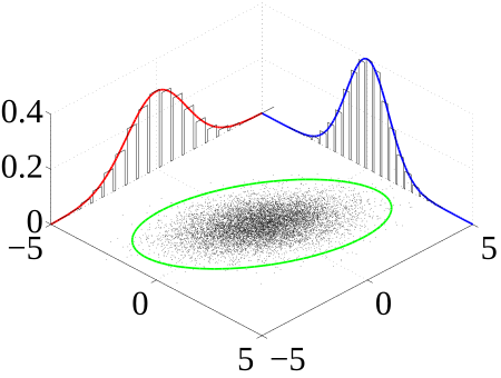
Many sample observations (black) are shown from a joint probability distribution. The marginal densities are shown as well.

The joint probability distribution can be expressed either in terms of a joint cumulative distribution function or in terms of a joint probability density function (in the case of continuous variables) or joint probability mass function (in the case of discrete variables). These in turn can be used to find two other types of distributions: the marginal distribution giving the probabilities for any one of the variables with no reference to any specific ranges of values for the other variables, and the conditional probability distribution giving the probabilities for any subset of the variables conditional on particular values of the remaining variables.

Discrete case

\[\begin{align} \mathrm{P}(X=x\ \mathrm{and}\ Y=y) = \mathrm{P}(Y=y \mid X=x) \cdot \mathrm{P}(X=x) = \mathrm{P}(X=x \mid Y=y) \cdot \mathrm{P}(Y=y) \end{align}\]

Continuous case

\[f_{X,Y}(x,y) = f_{Y\mid X}(y\mid x)f_X(x) = f_{X\mid Y}(x\mid y)f_Y(y)\;\]

Mixed case

\[\begin{align} f_{X,Y}(x,y) = f_{X \mid Y}(x \mid y)\mathrm{P}(Y=y)= \mathrm{P}(Y=y \mid X=x) f_X(x) \end{align}\]

Joint distribution for independent variables

$\ P(X = x \ \mbox{and} \ Y = y ) = P( X = x) \cdot P( Y = y)$
$\ f_{X,Y}(x,y) = f_X(x) \cdot f_Y(y)$

Sampling (statistics) @

In statistics, quality assurance, and survey methodology, sampling is concerned with the selection of a subset of individuals from within a statistical population to estimate characteristics of the whole population. Each observation measures one or more properties (such as weight, location, color) of observable bodies distinguished as independent objects or individuals. In survey sampling, weights can be applied to the data to adjust for the sample design, particularly stratified sampling. Results from probability theory and statistical theory are employed to guide the practice. In business and medical research, sampling is widely used for gathering information about a population.

The sampling process comprises several stages:

Defining the population of concern
Specifying a sampling frame, a set of items or events possible to measure
Specifying a sampling method for selecting items or events from the frame
Determining the sample size
Implementing the sampling plan
Sampling and data collecting
Data which can be selected

Survey methodology @

Statistical surveys are undertaken with a view towards making statistical inferences about the population being studied, and this depends strongly on the survey questions used. Polls about public opinion, public health surveys, market research surveys, government surveys and censuses are all examples of quantitative research that use contemporary survey methodology to answer questions about a population. Although censuses do not include a “sample”, they do include other aspects of survey methodology, like questionnaires, interviewers, and nonresponse follow-up techniques. Surveys provide important information for all kinds of public information and research fields, e.g., marketing research, psychology, health professionals and sociology.

Confidence interval @ @

In statistics, a confidence interval (CI) is a type of interval estimate of a population parameter. It is an observed interval (i.e., it is calculated from the observations), in principle different from sample to sample, that frequently includes the value of an unobservable parameter of interest if the experiment is repeated. How frequently the observed interval contains the parameter is determined by the confidence level or confidence coefficient. More specifically, the meaning of the term “confidence level” is that, if CI are constructed across many separate data analyses of replicated (and possibly different) experiments, the proportion of such intervals that contain the true value of the parameter will match the given confidence level. Whereas two-sided confidence limits form a confidence interval, their one-sided counterparts are referred to as lower/upper confidence bounds (or limits).

Let X be a random sample from a probability distribution with statistical parameters θ, which is a quantity to be estimated, and ϕ, representing quantities that are not of immediate interest. A confidence interval for the parameter θ, with confidence level or confidence coefficient γ, is an interval with random endpoints (u(X), v(X)), determined by the pair of random variables u(X) and v(X), with the property:

\[{\Pr}_{\theta,\phi}(u(X)<\theta<v(X))=\gamma\text{ for all }(\theta,\phi).\]

Fiducial inference @

Fiducial inference is one of a number of different types of statistical inference. These are rules, intended for general application, by which conclusions can be drawn from samples of data. In modern statistical practice, attempts to work with fiducial inference have fallen out of fashion in favour of frequentist inference, Bayesian inference and decision theory. However, fiducial inference is important in the history of statistics since its development led to the parallel development of concepts and tools in theoretical statistics that are widely used. Some current research in statistical methodology is either explicitly linked to fiducial inference or is closely connected to it.

Fiducial inference can be interpreted as an attempt to perform inverse probability without calling on prior probability distributions. Fiducial inference quickly attracted controversy and was never widely accepted. Indeed, counter-examples to the claims of Fisher for fiducial inference were soon published. These counter-examples cast doubt on the coherence of “fiducial inference” as a system of statistical inference or inductive logic. Other studies showed that, where the steps of fiducial inference are said to lead to “fiducial probabilities” (or “fiducial distributions”), these probabilities lack the property of additivity, and so cannot constitute a probability measure.

The concept of fiducial inference can be outlined by comparing its treatment of the problem of interval estimation in relation to other modes of statistical inference.

Fisher required the existence of a sufficient statistic for the fiducial method to apply. Suppose there is a single sufficient statistic for a single parameter. That is, suppose that the conditional distribution of the data given the statistic does not depend on the value of the parameter. For example suppose that n independent observations are uniformly distributed on the interval $[0,\omega]$. The maximum, X, of the n observations is a sufficient statistic for ω. If only X is recorded and the values of the remaining observations are forgotten, these remaining observations are equally likely to have had any values in the interval [0,X]. This statement does not depend on the value of ω. Then X contains all the available information about ω and the other observations could have given no further information.

The CDF of X is

\[F(x) = P(X \leq x) = P\left(\mathrm{all\ observations} \leq x\right) = \left(\frac{x}{\omega}\right)^n.\]

Probability statements about X/ω may be made. For example, given α, a value of a can be chosen with 0 < a < 1 such that

\[P\left(X > \frac{\omega }{a}\right) = 1-a^n = \alpha.\]

Thus

\[a = (1-\alpha)^{\frac{1}{n}}.\]

Then Fisher might say that this statement may be inverted into the form

\[P\left(\omega < \frac{X}{a}\right) = \alpha.\]

Pivotal quantity @

In statistics, a pivotal quantity or pivot is a function of observations and unobservable parameters whose probability distribution does not depend on the unknown parameters (also referred to as nuisance parameters). Note that a pivot quantity need not be a statistic—the function and its value can depend on the parameters of the model, but its distribution must not. If it is a statistic, then it is known as an ancillary statistic.

More formally, let $X = (X_1,X_2,\ldots,X_n)$ be a random sample from a distribution that depends on a parameter (or vector of parameters) $\theta$. Let $g(X,\theta)$ be a random variable whose distribution is the same for all $\theta$. Then g is called a pivotal quantity (or simply a pivot).

Pivotal quantities are commonly used for normalization to allow data from different data sets to be compared. It is relatively easy to construct pivots for location and scale parameters: for the former we form differences so that location cancels, for the latter ratios so that scale cancels.

Pivotal quantities are fundamental to the construction of test statistics, as they allow the statistic to not depend on parameters – for example, Student’s t-statistic is for a normal distribution with unknown variance (and mean). They also provide one method of constructing confidence intervals, and the use of pivotal quantities improves performance of the bootstrap. In the form of ancillary statistics, they can be used to construct frequentist prediction intervals (predictive confidence intervals).

One of the simplest pivotal quantities is the z-score; given a normal distribution with mean $\mu$ and variance $\sigma^2$, and an observation x, the z-score:

\[z = \frac{x - \mu}{\sigma},\]

has distribution N(0,1).

Regression analysis @

Least squares @

The minimum of the sum of squares is found by setting the gradient to zero. Since the model contains m parameters, there are m gradient equations:

\[\frac{\partial S}{\partial \beta_j}=2\sum_i r_i\frac{\partial r_i}{\partial \beta_j}=0,\ j=1,\ldots,m,\]

and since $r_i=y_i-f(x_i,\boldsymbol \beta)$, the gradient equations become

\[-2\sum_i r_i\frac{\partial f(x_i,\boldsymbol \beta)}{\partial \beta_j}=0,\ j=1,\ldots,m.\]

The gradient equations apply to all least squares problems. Each particular problem requires particular expressions for the model and its partial derivatives.

Linear least squares
Non-linear least squares
Weighted least squares

Gauss–Markov theorem

Linear regression @

In statistics, linear regression is an approach for modeling the relationship between a scalar dependent variable y and one or more explanatory variables (or independent variables) denoted X. The case of one explanatory variable is called simple linear regression. For more than one explanatory variable, the process is called multiple linear regression. (This term should be distinguished from multivariate linear regression, where multiple correlated dependent variables are predicted, rather than a single scalar variable.)

Given a data set $\{y_i,\, x_{i1}, \ldots, x_{ip}\}_{i=1}^n$ of n statistical units, a linear regression model assumes that the relationship between the dependent variable yi and the p-vector of regressors xi is linear. This relationship is modeled through a disturbance term or error variable $ε_i$ — an unobserved random variable that adds noise to the linear relationship between the dependent variable and regressors. Thus the model takes the form

\[y_i = \beta_1 x_{i1} + \cdots + \beta_p x_{ip} + \varepsilon_i = \mathbf{x}^{\rm T}_i\boldsymbol\beta + \varepsilon_i, \qquad i = 1, \ldots, n,\]

where T denotes the transpose, so that xiTβ is the inner product between vectors xi and β.

Often these n equations are stacked together and written in vector form as

\[\mathbf{y} = \mathbf{X}\boldsymbol\beta + \boldsymbol\varepsilon, \,\]

where

$\mathbf{y} = \begin{pmatrix} y_1 \\ y_2 \\ \vdots \\ y_n \end{pmatrix}, \quad$
$\mathbf{X} = \begin{pmatrix} \mathbf{x}^{\rm T}_1 \\ \mathbf{x}^{\rm T}_2 \\ \vdots \\ \mathbf{x}^{\rm T}_n \end{pmatrix} = \begin{pmatrix} x_{11} & \cdots & x_{1p} \\ x_{21} & \cdots & x_{2p} \\ \vdots & \ddots & \vdots \\ x_{n1} & \cdots & x_{np} \end{pmatrix},$
$\boldsymbol\beta = \begin{pmatrix} \beta_1 \\ \beta_2 \\ \vdots \\ \beta_p \end{pmatrix}, \quad \boldsymbol\varepsilon = \begin{pmatrix} \varepsilon_1 \\ \varepsilon_2 \\ \vdots \\ \varepsilon_n \end{pmatrix}.$

Nonlinear regression @

In statistics, nonlinear regression is a form of regression analysis in which observational data are modeled by a function which is a nonlinear combination of the model parameters and depends on one or more independent variables. The data are fitted by a method of successive approximations.

For example, the Michaelis–Menten model for enzyme kinetics

\[v = \frac{V_\max\ [\mbox{S}]}{K_m + [\mbox{S}]}\]

can be written as

\[f(x,\boldsymbol\beta)= \frac{\beta_1 x}{\beta_2 + x}\]

where $\beta_1$ is the parameter $V_\max$, $\beta_2$ is the parameter $K_m$ and $[S]$ is the independent variable, x. This function is nonlinear because it cannot be expressed as a linear combination of the two $\beta$s.

Other examples of nonlinear functions include exponential functions, logarithmic functions, trigonometric functions, power functions, Gaussian function, and Lorenz curves. Some functions, such as the exponential or logarithmic functions, can be transformed so that they are linear. When so transformed, standard linear regression can be performed but must be applied with caution. See Linearization, below, for more details.

See Michaelis-Menten kinetics for details.

Residual sum of squares @

In a model with a single explanatory variable, RSS is given by:

\[RSS = \sum_{i=1}^n (y_i - f(x_i))^2,\]

where yi is the i th value of the variable to be predicted, xi is the i th value of the explanatory variable, and f(x_i) is the predicted value of yi (also termed ). In a standard linear simple regression model, $y_i = a+bx_i+\varepsilon_i\,$, where a and b are coefficients, y and x are the regressand and the regressor, respectively, and ε is the error term. The sum of squares of residuals is the sum of squares of estimates of $ε_i$; that is

\[RSS = \sum_{i=1}^n (\varepsilon_i)^2 = \sum_{i=1}^n (y_i - (\alpha + \beta x_i))^2,\]

where is the estimated value of the constant term a and is the estimated value of the slope coefficient b.

Matrix expression for the OLS residual sum of squares

The general regression model with n observations and k explanators, the first of which is a constant unit vector whose coefficient is the regression intercept, is

\[y = X \beta + e\]

where y is an n × 1 vector of dependent variable observations, each column of the n × k matrix X is a vector of observations on one of the k explanators, is a k × 1 vector of true coefficients, and e is an n× 1 vector of the true underlying errors. The ordinary least squares estimator for is

\[\hat \beta = (X^T X)^{-1}X^T y.\]

The residual vector e is y - X = y - X (X^T X)^{-1}XT y, so the residual sum of squares is:

\[RSS = \hat e ^T \hat e = \| e \|^2,\]

(equivalent to the square-root of the norm of residuals); in full:

\[RSS = y^T y - y^T X(X^T X)^{-1} X^T y = y^T [I - X(X^T X)^{-1} X^T] y = y^T [I - H] y,\]

where H is the hat matrix, or the prediction matrix in linear regression.

Projection matrix - Wikipedia, the free encyclopedia

In statistics, the projection matrix $\mathbf{P}$, sometimes also called the influence matrix or hat matrix $\mathbf{H}$, maps the vector of response values (dependent variable values) to the vector of fitted values (or predicted values). It describes the influence each response value has on each fitted value. The diagonal elements of the projection matrix are the leverages, which describe the influence each response value has on the fitted value for that same observation.

If the vector of response values is denoted by $\mathbf{y}$ and the vector of fitted values by $\mathbf{\hat{y}}$,

\[ \mathbf{\hat{y}} = \mathbf{P} \mathbf{y}. \]

As $\mathbf{\hat{y}}$ is usually pronounced “y-hat”, the projection matrix is also named hat matrix as it “puts a hat on $\mathbf{y}$”. The formula for the vector of residuals $\mathbf{u}$ can also be expressed compactly using the projection matrix:

\[ \mathbf{u} = \mathbf{y} - \mathbf{\hat{y}} = \mathbf{y} - \mathbf{P} \mathbf{y} = \left( \mathbf{I} - \mathbf{P} \right) \mathbf{y}. \]

where $\mathbf{I}$ is the identity matrix. The matrix $\mathbf{M} \equiv \left( \mathbf{I} - \mathbf{P} \right)$ is sometimes referred to as annihilator. Moreover, the element in the ith row and jth column of $\mathbf{P}$ is equal to the covariance between the jth response value and the ith fitted value, divided by the variance of the former:

\[ \begin{align} p_{ij} = \operatorname{Cov}\left[ \hat{y}_i, y_j \right] / \operatorname{Var}\left[y_j \right] \end{align} \]

Therefore, the covariance matrix of the residuals, by error propagation, equals $\left( \mathbf{I}-\mathbf{P} \right)^{\mathsf{T}} \mathbf{\Sigma} \left( \mathbf{I}-\mathbf{P} \right)$, where $\mathbf{\Sigma}$ is the covariance matrix of the error vector (and by extension, the response vector as well). For the case of linear models with independent and identically distributed errors in which $\mathbf{\Sigma} = \sigma^{2} \mathbf{I}$, this reduces to $\left( \mathbf{I} - \mathbf{P} \right) \sigma^{2}$.

Ordinary least squares @

普通最小二乘法

In statistics, ordinary least squares (OLS) or linear least squares is a method for estimating the unknown parameters in a linear regression model, with the goal of minimizing the differences between the observed responses in some arbitrary dataset and the responses predicted by the linear approximation of the data (visually this is seen as the sum of the vertical distances between each data point in the set and the corresponding point on the regression line - the smaller the differences, the better the model fits the data). The resulting estimator can be expressed by a simple formula, especially in the case of a single regressor on the right-hand side.

\[y = X\beta + \varepsilon, \,\]

where y and ε are n×1 vectors, and X is an n×p matrix of regressors, which is also sometimes called the design matrix.

regressors, 回归因子选择；回归数值。

Classical linear regression model

Correct specification. The linear functional form is correctly specified.
Strict exogeneity (外生性). The errors in the regression should have conditional mean zero:

\[\operatorname{E}[\,\varepsilon|X\,] = 0.\]
No linear dependence. The regressors in X must all be linearly independent. Mathematically, this means that the matrix X must have full column rank almost surely: （意思是所选参数都是有效的。）

\[\Pr\!\big[\,\operatorname{rank}(X) = p\,\big] = 1.\]
Spherical errors:（意思是误差均匀分布在各个方向上）

\[\operatorname{Var}[\,\varepsilon \mid X\,] = \sigma^2 I_n,\]
Normality. It is sometimes additionally assumed that the errors have normal distribution conditional on the regressors:

\[\varepsilon \mid X\sim \mathcal{N}(0, \sigma^2I_n).\]

The sum of squared residuals (SSR) (also called the error sum of squares (ESS) or residual sum of squares (RSS)) is a measure of the overall model fit:

\[ S(b) = \sum_{i=1}^n (y_i - x_i ^T b)^2 = (y-Xb)^T(y-Xb), \]

where T denotes the matrix transpose.

Geometric approach

OLS estimation can be viewed as a projection onto the linear space spanned by the regressors.

\[\hat\beta = {\rm arg}\min_\beta\,\lVert y - X\beta \rVert,\]

Maximum likelihood

The OLS estimator is identical to the maximum likelihood estimator (MLE) under the normality assumption for the error terms.

see at #maximum-likelihood.

Generalized method of moments

In iid case the OLS estimator can also be viewed as a GMM estimator arising from the moment conditions

\[\mathrm{E}\big[\, x_i(y_i - x_i ^T \beta) \,\big] = 0.\]

First of all, under the strict exogeneity assumption the OLS estimators $\scriptstyle\hat\beta$ and $s^2$ are unbiased, meaning that their expected values coincide with the true values of the parameters:

\[\operatorname{E}[\, \hat\beta \mid X \,] = \beta, \quad \operatorname{E}[\,s^2 \mid X\,] = \sigma^2.\]

The estimator $\scriptstyle\hat\beta$ is normally distributed, with mean and variance as given before:

\[\hat\beta\ \sim\ \mathcal{N}\big(\beta,\ \sigma^2(X ^T X)^{-1}\big)\]

The estimator $s^2$ will be proportional to the chi-squared distribution:

\[s^2\ \sim\ \frac{\sigma^2}{n-p} \cdot \chi^2_{n-p}\]

Generalized method of moments @ @

In econometrics, the generalized method of moments (GMM) is a generic method for estimating parameters in statistical models. Usually it is applied in the context of semiparametric models, where the parameter of interest is finite-dimensional, whereas the full shape of the distribution function of the data may not be known, and therefore maximum likelihood estimation is not applicable.

The method requires that a certain number of moment conditions were specified for the model. These moment conditions are functions of the model parameters and the data, such that their expectation is zero at the true values of the parameters. The GMM method then minimizes a certain norm of the sample averages of the moment conditions.

The GMM estimators are known to be consistent, asymptotically (渐进地) normal, and efficient in the class of all estimators that do not use any extra information aside from that contained in the moment conditions.

GMM was developed by Lars Peter Hansen in 1982 as a generalization of the method of moments which was introduced by Karl Pearson in 1894. Hansen shared the 2013 Nobel Prize in Economics in part for this work.

这么叼……三十年前的工作……。

Nonparametric regression @

Gaussian process regression or Kriging @

see Kriging - Wikipedia, the free encyclopedia.

In statistics, originally in geostatistics, Kriging or Gaussian process regression is a method of interpolation for which the interpolated values are modeled by a Gaussian process governed by prior covariances, as opposed to a piecewise-polynomial spline chosen to optimize smoothness of the fitted values. Under suitable assumptions on the priors, Kriging gives the best linear unbiased prediction of the intermediate values. Interpolating methods based on other criteria such as smoothness need not yield the most likely intermediate values. The method is widely used in the domain of spatial analysis and computer experiments. The technique is also known as Wiener–Kolmogorov prediction, after Norbert Wiener and Andrey Kolmogorov.

The theoretical basis for the method was developed by the French mathematician Georges Matheron based on the Master’s thesis of Danie G. Krige, the pioneering plotter of distance-weighted average gold grades at the Witwatersrand reef complex in South Africa. Krige sought to estimate the most likely distribution of gold based on samples from a few boreholes. The English verb is to krige and the most common noun is Kriging; both are often pronounced with a hard “g”, following the pronunciation of the name “Krige”.

Example of one-dimensional data interpolation by Kriging, with confidence intervals. Squares indicate the location of the data. The Kriging interpolation, shown in red, runs along the means of the normally distributed confidence intervals shown in gray. The dashed curve shows a spline that while smooth nevertheless departs significantly from the expected intermediate values given by those means.

Kernel regression

Nonparametric multiplicative regression (NPMR) is a form of nonparametric regression based on multiplicative kernel estimation. Like other regression methods, the goal is to estimate a response (dependent variable) based on one or more predictors (independent variables). NPMR can be a good choice for a regression method if the following are true:

The shape of the response surface is unknown.
The predictors are likely to interact in producing the response; in other words, the shape of the response to one predictor is likely to depend on other predictors.
The response is either a quantitative or binary (0/1) variable.

This is a smoothing technique that can be cross-validated and applied in a predictive way.

NPMR behaves like an organism:

The local model
Overfitting controls

Regression trees

Least absolute deviations @

Least absolute deviations (LAD), also known as least absolute errors (LAE), least absolute value (LAV), least absolute residual (LAR), sum of absolute deviations, or the L1 norm condition, is a statistical optimality criterion and the statistical optimization technique that relies on it. Similar to the popular least squares technique, it attempts to find a function which closely approximates a set of data. In the simple case of a set of (x,y) data, the approximation function is a simple “trend line” in two-dimensional Cartesian coordinates. The method minimizes the sum of absolute errors (SAE) (the sum of the absolute values of the vertical “residuals” between points generated by the function and corresponding points in the data). The least absolute deviations estimate also arises as the maximum likelihood estimate if the errors have a Laplace distribution.

We now seek estimated values of the unknown parameters that minimize the sum of the absolute values of the residuals:

\[S = \sum_{i=1}^n |y_i - f(x_i)|. \]

Least squares regression	Least absolute deviations regression
Not very robust	Robust
Stable solution	Unstable solution
Always one solution	Possibly multiple solutions

Bias of an estimator @

TODO: Bias of an estimator - Wikipedia, the free encyclopedia

In statistics, the bias (or bias function) of an estimator is the difference between this estimator’s expected value and the true value of the parameter being estimated. An estimator or decision rule with zero bias is called unbiased. Otherwise the estimator is said to be biased.

In statistics, “bias” is an objective statement about a function, and while not a desired property, it is not pejorative, unlike the ordinary English use of the term “bias”. (这还解释，显示好人文关怀。)

Bias can also be measured with respect to the median, rather than the mean (expected value), in which case one distinguishes median-unbiased from the usual mean-unbiasedness property. Bias is related to consistency in that consistent estimators are convergent and asymptotically unbiased (hence converge to the correct value), though individual estimators in a consistent sequence may be biased (so long as the bias converges to zero); see bias versus consistency.

All else equal, an unbiased estimator is preferable to a biased estimator, but in practice all else is not equal, and biased estimators are frequently used, generally with small bias. When a biased estimator is used, the bias is also estimated. A biased estimator may be used for various reasons: because an unbiased estimator does not exist without further assumptions about a population or is difficult to compute (as in unbiased estimation of standard deviation); because an estimator is median-unbiased but not mean-unbiased (or the reverse); because a biased estimator reduces some loss function (particularly mean squared error) compared with unbiased estimators (notably in shrinkage 收缩程度 estimators); or because in some cases being unbiased is too strong a condition, and the only unbiased estimators are not useful. Further, mean-unbiasedness is not preserved under non-linear transformations, though median-unbiasedness is (see effect of transformations); for example, the sample variance is an unbiased estimator for the population variance, but its square root, the sample standard deviation, is a biased estimator for the population standard deviation.

\[ \operatorname{Bias}_\theta[\,\hat\theta\,] = \operatorname{E}_\theta[\,\hat{\theta}\,]-\theta = \operatorname{E}_\theta[\, \hat\theta - \theta \,], \]

If the sample mean and uncorrected sample variance are defined as

\[ \overline{X}=\frac{1}{n}\sum_{i=1}^nX_i, \qquad S^2=\frac{1}{n}\sum_{i=1}^n\left(X_i-\overline{X}\,\right)^2, \]

then $S^2$ is a biased estimator of σ2.

Efficient estimator @

In statistics, an efficient estimator is an estimator that estimates the quantity of interest in some “best possible” manner. The notion of “best possible” relies upon the choice of a particular loss function — the function which quantifies the relative degree of undesirability of estimation errors of different magnitudes. The most common choice of the loss function is quadratic, resulting in the mean squared error criterion of optimality.

有效估计量是相对的，可以说一个估计量比另一个有效，那么它是有效估计量。也可以说在某一损失函数下最有效的那个估计量是有效估计量（比其他都有效）。

TODO: Efficient estimator - Wikipedia, the free encyclopedia

Consistent estimator @

In statistics, a consistent estimator or asymptotically consistent estimator is an estimator—a rule for computing estimates of a parameter θ0— having the property that as the number of data points used increases indefinitely, the resulting sequence of estimates converges in probability to θ0. This means that the distributions of the estimates become more and more concentrated near the true value of the parameter being estimated, so that the probability of the estimator being arbitrarily close to θ0 converges to one.

很多统计书里会翻译成“一致统计量”，其实是“持续”统计量。意思是能够不断逼近期望，随着样本数量的增多，这个估计策略一定会越来越靠谱。

{T1, T2, T3, …} is a sequence of estimators for parameter θ0, the true value of which is 4. This sequence is consistent: the estimators are getting more and more concentrated near the true value θ0; at the same time, these estimators are biased. The limiting distribution of the sequence is a degenerate random variable which equals θ0 with probability 1.

Bias versus consistency

Bias is related to consistency as follows: a sequence of estimators is consistent if and only if it converges to a value and the bias converges to zero.

Unbiased but not consistent

Biased but consistent

Observational error @

Observational error (or measurement error) is the difference between a measured value of quantity and its true value. In statistics, an error is not a “mistake”. Variability is an inherent part of things being measured and of the measurement process.

Measurement errors can be divided into two components: random error and systematic error. Random errors are errors in measurement that lead to measurable values being inconsistent when repeated measures of a constant attribute or quantity are taken. Systematic errors are errors that are not determined by chance but are introduced by an inaccuracy (as of observation or measurement) inherent in the system. Systematic error may also refer to an error having a nonzero mean, so that its effect is not reduced when observations are averaged.

Systematic versus random error

Sources of systematic error

Imperfect calibration
Quantity

Systematic errors can be either constant, or related (e.g. proportional or a percentage) to the actual value of the measured quantity, or even to the value of a different quantity
Drift

Sources of random error @

The random or stochastic error in a measurement is the error that is random from one measurement to the next. Stochastic errors tend to be normally distributed when the stochastic error is the sum of many independent random errors because of the central limit theorem. Stochastic errors added to a regression equation account for the variation in Y that cannot be explained by the included Xs.

The term “observational error” is also sometimes used to refer to response errors and some other types of non-sampling error. In survey-type situations, these errors can be mistakes in the collection of data, including both the incorrect recording of a response and the correct recording of a respondent’s inaccurate response. These sources of non-sampling error are discussed in Salant and Dillman (1995) and Bland and Altman (1996).

Stochastic process - Wikipedia, the free encyclopedia @

In probability theory, a stochastic (/stoʊˈkæstɪk/) process, or often random process, is a collection of random variables representing the evolution of some system of random values over time. This is the probabilistic counterpart to a deterministic process (or deterministic system). Instead of describing a process which can only evolve in one way (as in the case, for example, of solutions of an ordinary differential equation), in a stochastic, or random process, there is some indeterminacy: even if the initial condition (or starting point) is known, there are several (often infinitely many) directions in which the process may evolve.

In the simple case of discrete time, as opposed to continuous time, a stochastic process is a sequence of random variables. (For example, see Markov chain, also known as discrete-time Markov chain.) The random variables corresponding to various times may be completely different, the only requirement being that these different random quantities all take values in the same space (the codomain of the function). One approach may be to model these random variables as random functions of one or several deterministic arguments (in most cases, the time parameter). Although the random values of a stochastic process at different times may be independent random variables, in most commonly considered situations they exhibit complicated statistical dependence.

Familiar examples of stochastic processes include stock market and exchange rate fluctuations; signals such as speech; audio and video; medical data such as a patient’s EKG, EEG, blood pressure or temperature; and random movement such as Brownian motion or random walks.

A generalization, the random field, is defined by letting the variables be parametrized by members of a topological space instead of time. Examples of random fields include static images, random terrain (landscapes), wind waves and composition variations of a heterogeneous material.

Stock market fluctuations have been modeled by stochastic processes.

Estimator @

In statistics, an estimator is a rule for calculating an estimate of a given quantity based on observed data: thus the rule (the estimator), the quantity of interest (the estimand) and its result (the estimate) are distinguished.

There are point and interval estimators. The point estimators yield single-valued results, although this includes the possibility of single vector-valued results and results that can be expressed as a single function. This is in contrast to an interval estimator, where the result would be a range of plausible values (or vectors or functions).

Estimation theory is concerned with the properties of estimators; that is, with defining properties that can be used to compare different estimators (different rules for creating estimates) for the same quantity, based on the same data. Such properties can be used to determine the best rules to use under given circumstances. However, in robust statistics, statistical theory goes on to consider the balance between having good properties, if tightly defined assumptions hold, and having less good properties that hold under wider conditions.

Point estimation @

In statistics, point estimation involves the use of sample data to calculate a single value (known as a statistic) which is to serve as a “best guess” or “best estimate” of an unknown (fixed or random) population parameter.

More formally, it is the application of a point estimator to the data.

In general, point estimation should be contrasted with interval estimation: such interval estimates are typically either confidence intervals in the case of frequentist inference, or credible intervals in the case of Bayesian inference.

Point estimators

minimum-variance mean-unbiased estimator (MVUE)

minimizes the risk (expected loss) of the squared-error loss-function.

In statistics a uniformly minimum-variance unbiased estimator or minimum-variance unbiased estimator (UMVUE or MVUE) is an unbiased estimator that has lower variance than any other unbiased estimator for all possible values of the parameter.

For a normal distribution with unknown mean and variance, the sample mean and (unbiased) sample variance are the MVUEs for the population mean and population variance.
best linear unbiased estimator (BLUE)

In statistics, the Gauss–Markov theorem, named after Carl Friedrich Gauss and Andrey Markov, states that in a linear regression model in which the errors have expectation zero and are uncorrelated and have equal variances, the best linear unbiased estimator (BLUE) of the coefficients is given by the ordinary least squares (OLS) estimator. Here “best” means giving the lowest variance of the estimate, as compared to other unbiased, linear estimators. The errors do not need to be normal, nor do they need to be independent and identically distributed (only uncorrelated with mean zero and homoscedastic with finite variance). The requirement that the estimator be unbiased cannot be dropped, since biased estimators exist with lower variance. See, for example, the James–Stein estimator (which also drops linearity) or ridge regression.

The Gauss–Markov assumptions are
- $E(\varepsilon_i)=0$,
- $V(\varepsilon_i)= \sigma^2 < \infty$,
(i.e., all disturbances have the same variance; that is “homoscedasticity”⁴), and

\[{\rm cov}(\varepsilon_i,\varepsilon_j) = 0, \forall i \neq j\]
minimum mean squared error (MMSE)

In statistics and signal processing, a minimum mean square error (MMSE) estimator is an estimation method which minimizes the mean square error (MSE), which is a common measure of estimator quality, of the fitted values of a dependent variable. In the Bayesian setting, the term MMSE more specifically refers to estimation with quadratic cost function. In such case, the MMSE estimator is given by the posterior mean of the parameter to be estimated. Since the posterior mean is cumbersome to calculate, the form of the MMSE estimator is usually constrained to be within a certain class of functions. Linear MMSE estimators are a popular choice since they are easy to use, calculate, and very versatile. It has given rise to many popular estimators such as the Wiener-Kolmogorov filter and Kalman filter.

Let x be a n $\times$ 1 hidden random vector variable, and let y be a m $\times$ 1 known random vector variable (the measurement or observation), both of them not necessarily of the same dimension. An estimator $\hat{x}(y)$ of x is any function of the measurement y. The estimation error vector is given by $e = \hat{x} - x$ and its mean squared error (MSE) is given by the trace of error covariance matrix

\[\mathrm{MSE} = \mathrm{tr} \left\{ \mathrm{E}\{(\hat{x} - x)(\hat{x} - x)^T \}\right\},\]

where the expectation $\mathrm{E}$ is taken over both x and y. When x is a scalar variable, the MSE expression simplifies to $\mathrm{E}$ $\left\{ (\hat{x} - x)^2 \right\}$. Note that MSE can equivalently be defined in other ways, since

\[\mathrm{tr} \left\{ \mathrm{E}\{ee^T \} \right\} = \mathrm{E} \left\{ \mathrm{tr}\{ee^T \} \right\} = \mathrm{E}\{e^T e \} = \sum_{i=1}^n \mathrm{E}\{e_i^2\}.\]

The MMSE estimator is then defined as the estimator achieving minimal MSE:

\[\hat{x}_{\mathrm{MMSE}}(y) = \arg \min_{\hat{x}} \mathrm{MSE}.\]
median-unbiased estimator

Any mean-unbiased estimator minimizes the risk (expected loss) with respect to the squared-error loss function, as observed by Gauss. A median-unbiased estimator minimizes the risk with respect to the absolute-deviation loss function, as observed by Laplace. Other loss functions are used in statistical theory, particularly in robust statistics.
maximum likelihood (ML)

see more at #maximum-likelihood.
method of moments, generalized method of moments

Bayesian point-estimation @

Bayesian inference is typically based on the posterior distribution. Many Bayesian point-estimators are the posterior distribution’s statistics of central tendency, e.g., its mean, median, or mode:

Posterior mean, which minimizes the (posterior) risk (expected loss) for a squared-error loss function; in Bayesian estimation, the risk is defined in terms of the posterior distribution.
Posterior median, which minimizes the posterior risk for the absolute-value loss function.
maximum a posteriori (MAP), which finds a maximum of the posterior distribution; for a uniform prior probability, the MAP estimator coincides with the maximum-likelihood estimator;

The MAP estimator has good asymptotic properties, even for many difficult problems, on which the maximum-likelihood estimator has difficulties. For regular problems, where the maximum-likelihood estimator is consistent, the maximum-likelihood estimator ultimately agrees with the MAP estimator. Bayesian estimators are admissible, by Wald’s theorem.

The Minimum Message Length (MML) point estimator is based in Bayesian information theory and is not so directly related to the posterior distribution.

Special cases of Bayesian estimators are important:

Kalman filter
Wiener filter

Several methods of computational statistics have close connections with Bayesian analysis:

particle filter Markov chain Monte Carlo (MCMC)

Properties of point estimates

bias of an estimator⁵
Cramér–Rao bound

Interval estimation @

In statistics, interval estimation is the use of sample data to calculate an interval of possible (or probable) values of an unknown population parameter, in contrast to point estimation, which is a single number. Jerzy Neyman (1937) identified interval estimation (“estimation by interval”) as distinct from point estimation (“estimation by unique estimate”). In doing so, he recognised that then-recent work quoting results in the form of an estimate plus-or-minus a standard deviation indicated that interval estimation was actually the problem statisticians really had in mind.

The most prevalent forms of interval estimation are:

confidence intervals (a frequentist method); and
credible intervals (a Bayesian method).

Other common approaches to interval estimation, which are encompassed by statistical theory, are:

Tolerance intervals
Prediction intervals - used mainly in Regression Analysis
Likelihood intervals

There is another approach to statistical inference, namely fiducial inference, that also considers interval estimation. Non-statistical methods that can lead to interval estimates include fuzzy logic.

An interval estimate is one type of outcome of a statistical analysis. Some other types of outcome are point estimates and decisions.

Kalman filter @

$The Kalman filter keeps track of the estimated state of the system and the variance or uncertainty of the estimate. The estimate is updated using a state transition model and measurements. \hat{x}_{k\mid k-1} denotes the estimate of the system’s state at time step k before the k-th measurement yk has been taken into account; P_{k\mid k-1} is the corresponding uncertainty.$

The Kalman filter keeps track of the estimated state of the system and the variance or uncertainty of the estimate. The estimate is updated using a state transition model and measurements. $\hat{x}_{k\mid k-1}$ denotes the estimate of the system’s state at time step k before the k-th measurement yk has been taken into account; $P_{k\mid k-1}$ is the corresponding uncertainty.

TODO

Wiener filter @

TODO

Bayesian statistics @

Bayesian statistics, named for Thomas Bayes (1701-1761), is a theory in the field of statistics in which the evidence about the true state of the world is expressed in terms of ‘degrees of belief’ called Bayesian probabilities. Such an interpretation is only one of a number of interpretations of probability and there are other statistical techniques that are not based on ‘degrees of belief’. One of the key ideas of Bayesian statistics is that “probability is orderly opinion, and that inference from data is nothing other than the revision of such opinion in the light of relevant new information.”

Bayesian linear regression @

In statistics, Bayesian linear regression is an approach to linear regression in which the statistical analysis is undertaken within the context of Bayesian inference. When the regression model has errors that have a normal distribution, and if a particular form of prior distribution is assumed, explicit results are available for the posterior probability distributions of the model’s parameters.

Model setup @

Consider a standard linear regression problem, in which for $i=1,...,n$ we specify the conditional distribution of $y_i$ given a k $\times$ 1 predictor vector $\mathbf{x}_i$:

\[y_{i} = \mathbf{x}_{i}^{\rm T} \boldsymbol\beta + \epsilon_{i},\]

where $\boldsymbol\beta$ is a k $\times$ 1 vector, and the $\epsilon_i$ are iid, and $\epsilon_{i} \sim N(0, \sigma^2).$

This corresponds to the following likelihood function:

\[\rho(\mathbf{y}|\mathbf{X},\boldsymbol\beta,\sigma^{2}) \propto (\sigma^{2})^{-n/2} \exp\left(-\frac{1}{2{\sigma}^{2}}(\mathbf{y}- \mathbf{X} \boldsymbol\beta)^{\rm T}(\mathbf{y}- \mathbf{X} \boldsymbol\beta)\right).\]

The ordinary least squares solution is to estimate the coefficient vector using the Moore-Penrose pseudoinverse:

\[\hat{\boldsymbol\beta} = (\mathbf{X}^{\rm T}\mathbf{X})^{-1}\mathbf{X}^{\rm T}\mathbf{y}\]

where $\mathbf{X}$ is the n $\times$ k design matrix, each row of which is a predictor vector $\mathbf{x}_{i}^{\rm T}$; and $\mathbf{y}$ is the column n-vector $[y_1 \; \cdots \; y_n]^{\rm T}$.

This is a frequentist approach, and it assumes that there are enough measurements to say something meaningful about $\boldsymbol\beta$. In the Bayesian approach, the data are supplemented with additional information in the form of a prior probability distribution. The prior belief about the parameters is combined with the data’s likelihood function according to Bayes theorem to yield the posterior belief about the parameters $\boldsymbol\beta$ and $\sigma$. The prior can take different functional forms depending on the domain and the information that is available a priori.

With conjugate priors @

For an arbitrary prior distribution, there may be no analytical solution for the posterior distribution. In this section, we will consider a so-called conjugate prior for which the posterior distribution can be derived analytically.

A prior $\rho$($\boldsymbol\beta,\sigma^{2}$) is conjugate to this likelihood function if it has the same functional form with respect to $\boldsymbol\beta$ and $\sigma$. Since the log-likelihood is quadratic in $\boldsymbol\beta$, the log-likelihood is re-written such that the likelihood becomes normal in ($\boldsymbol\beta-\hat{\boldsymbol\beta}$).

TODO

Bayesian linear regression - Wikipedia, the free encyclopedia

Model evidence: The model evidence p($\mathbf{y}|m$) is the probability of the data given the model m. It is also known as the marginal likelihood, and as the prior predictive density.

Statistical modeling @

The formulation of statistical models using Bayesian statistics has the unique feature of requiring the specification of prior distributions for any unknown parameters. These prior distributions are as integral to a Bayesian approach to statistical modelling as the expression of probability distributions. Prior distributions can be either hyperparameters or hyperprior distributions.

Bayesian inference @

Bayesian inference is a method of statistical inference in which Bayes’ theorem is used to update the probability for a hypothesis as more evidence or information becomes available. Bayesian inference is an important technique in statistics, and especially in mathematical statistics. Bayesian updating is particularly important in the dynamic analysis of a sequence of data. Bayesian inference has found application in a wide range of activities, including science, engineering, philosophy, medicine, sport, and law. In the philosophy of decision theory, Bayesian inference is closely related to subjective probability, often called “Bayesian probability”.

$A geometric visualisation of Bayes’ theorem. In the table, the values w, x, y and z give the relative weights of each corresponding condition and case. The figures denote the cells of the table involved in each metric, the probability being the fraction of each figure that is shaded. This shows that P(A|B) P(B) = P(B|A) P(A) i.e. P(A|B) = P(B|A) P(A)/P(B) . Similar reasoning can be used to show that P(Ā|B) = P(B|Ā) P(Ā)/P(B) etc.$

A geometric visualisation of Bayes’ theorem. In the table, the values w, x, y and z give the relative weights of each corresponding condition and case. The figures denote the cells of the table involved in each metric, the probability being the fraction of each figure that is shaded. This shows that P(A|B) P(B) = P(B|A) P(A) i.e. P(A|B) = P(B|A) P(A)/P(B) . Similar reasoning can be used to show that P(Ā|B) = P(B|Ā) P(Ā)/P(B) etc.

Formal @

Bayesian inference derives the posterior probability as a consequence of two antecedents, a prior probability and a “likelihood function” derived from a statistical model for the observed data. Bayesian inference computes the posterior probability according to Bayes’ theorem:

\[P(H\mid E) = \frac{P(E\mid H) \cdot P(H)}{P(E)}\]

where

$\textstyle \mid$ denotes a conditional probability;
$\textstyle H$ stands for any hypothesis whose probability may be affected by data (called evidence below). Often there are competing hypotheses, from which one chooses the most probable. the evidence $\textstyle E$ corresponds to new data that were not used in computing the prior probability.
$\textstyle P(H)$, the prior probability
$\textstyle P(H\mid E)$, the posterior probability
$\textstyle P(E\mid H)$ is the probability of observing $\textstyle E$ given $\textstyle H$.
$\textstyle P(E)$ is sometimes termed the marginal likelihood or “model evidence”. This factor is the same for all possible hypotheses being considered. (This can be seen by the fact that the hypothesis $\textstyle H$ does not appear anywhere in the symbol, unlike for all the other factors.) This means that this factor does not enter into determining the relative probabilities of different hypotheses.

Note that Bayes’ rule can also be written as follows:

\[P(H\mid E) = \frac{P(E\mid H)}{P(E)} \cdot P(H)\]

where the factor $\textstyle \frac{P(E\mid H)}{P(E)}$ represents the impact of E on the probability of H.

Informal @

If the evidence does not match up with a hypothesis, one should reject the hypothesis. But if a hypothesis is extremely unlikely a priori, one should also reject it, even if the evidence does appear to match up.

The critical point about Bayesian inference, then, is that it provides a principled way of combining new evidence with prior beliefs, through the application of Bayes’ rule. (Contrast this with frequentist inference, which relies only on the evidence as a whole, with no reference to prior beliefs.) Furthermore, Bayes’ rule can be applied iteratively: after observing some evidence, the resulting posterior probability can then be treated as a prior probability, and a new posterior probability computed from new evidence. This allows for Bayesian principles to be applied to various kinds of evidence, whether viewed all at once or over time. This procedure is termed “Bayesian updating”.

Alternatives to Bayesian updating

Dutch book
“probability kinematics”

TODO

Formal description of Bayesian inference @

Definitions

x, a data point in general. This may in fact be a vector of values.
$\theta$, the parameter of the data point’s distribution, i.e., $x \sim p(x \mid \theta)$. This may in fact be a vector of parameters.
$\alpha$, the hyperparameter⁶ of the parameter, i.e., $\theta \sim p(\theta \mid \alpha)$. This may in fact be a vector of hyperparameters.
$\mathbf{X}$, a set of n observed data points, i.e., $x_1,\ldots,x_n$.
$\tilde{x}$, a new data point whose distribution is to be predicted.

Bayesian inference

Bayesian prediction

The posterior predictive distribution is the distribution of a new data point, marginalized over the posterior:

\[p(\tilde{x} \mid \mathbf{X},\alpha) = \int_{\theta} p(\tilde{x} \mid \theta) p(\theta \mid \mathbf{X},\alpha) \operatorname{d}\!\theta\]
The prior predictive distribution is the distribution of a new data point, marginalized over the prior:

\[p(\tilde{x} \mid \alpha) = \int_{\theta} p(\tilde{x} \mid \theta) p(\theta \mid \alpha) \operatorname{d}\!\theta\]

Bayesian inference @ @

The prior distribution is the distribution of the parameter(s) before any data is observed, i.e. p() .

Naive Bayes spam filtering @

TODO, Naive Bayes spam filtering - Wikipedia, the free encyclopedia

\[\Pr(S|W) = \frac{\Pr(W|S) \cdot \Pr(S)}{\Pr(W|S) \cdot \Pr(S) + \Pr(W|H) \cdot \Pr(H)}\]

where:

$\Pr(S|W)$ is the probability that a message is a spam, knowing that the word “replica” is in it;
$\Pr(S)$ is the overall probability that any given message is spam;
$\Pr(W|S)$ is the probability that the word “replica” appears in spam messages;
$\Pr(H)$ is the overall probability that any given message is not spam (is “ham”);
$\Pr(W|H)$ is the probability that the word “replica” appears in ham messages.

The spamicity of a word

“what percentage of occurrences of the word”replica" appear in spam messages?"
This quantity is called “spamicity” (or “spaminess”) of the word “replica”, and can be computed.

Statistical hypothesis testing @ @

Statistical hypothesis testing is a key technique of both frequentist inference and Bayesian inference, although the two types of inference have notable differences. Statistical hypothesis tests define a procedure that controls (fixes) the probability of incorrectly deciding that a default position (null hypothesis) is incorrect. The procedure is based on how likely it would be for a set of observations to occur if the null hypothesis were true. Note that this probability of making an incorrect decision is not the probability that the null hypothesis is true, nor whether any specific alternative hypothesis is true. This contrasts with other possible techniques of decision theory in which the null and alternative hypothesis are treated on a more equal basis.

The testing process

null and alternative hypotheses
consider the statistical assumptions
state the relevant test statistic T
significance level (α)
Compute from the observations the observed value tobs of the test statistic T

An alternative process is commonly used:

Calculate the p-value

If the p-value is less than the required significance level (equivalently, if the observed test statistic is in the critical region), then we say the null hypothesis is rejected at the given level of significance. Rejection of the null hypothesis is a conclusion. This is like a “guilty” verdict in a criminal trial: the evidence is sufficient to reject innocence, thus proving guilt. We might accept the alternative hypothesis (and the research hypothesis).

Fisher popularized the “significance test”. He required a null-hypothesis (corresponding to a population frequency distribution) and a sample. His (now familiar) calculations determined whether to reject the null-hypothesis or not. Significance testing did not utilize an alternative hypothesis so there was no concept of a Type II error.

Significance test @

see Statistical hypothesis testing

Z-test @

TODO

Student’s t-test @

TODO

Bootstrapping (statistics) @

In statistics, bootstrapping can refer to any test or metric that relies on random sampling with replacement. Bootstrapping allows assigning measures of accuracy (defined in terms of bias, variance, confidence intervals, prediction error or some other such measure) to sample estimates. This technique allows estimation of the sampling distribution of almost any statistic using random sampling methods. Generally, it falls in the broader class of resampling methods.

A great advantage of bootstrap is its simplicity. It is a straightforward way to derive estimates of standard errors and confidence intervals for complex estimators of complex parameters of the distribution, such as percentile points, proportions, odds ratio, and correlation coefficients. Bootstrap is also an appropriate way to control and check the stability of the results. Although for most problems it is impossible to know the true confidence interval, bootstrap is asymptotically more accurate than the standard intervals obtained using sample variance and assumptions of normality.

Although bootstrapping is (under some conditions) asymptotically (逐渐地) consistent, it does not provide general finite-sample guarantees. The apparent simplicity may conceal the fact that important assumptions are being made when undertaking the bootstrap analysis (e.g. independence of samples) where these would be more formally stated in other approaches.

Percentile - Wikipedia, the free encyclopedia @

A percentile (or a centile) is a measure used in statistics indicating the value below which a given percentage of observations in a group of observations fall. For example, the 20th percentile is the value (or score) below which 20% of the observations may be found.

The 25th percentile is also known as the first quartile (Q1), the 50th percentile as the median or second quartile (Q2), and the 75th percentile as the third quartile (Q3). In general, percentiles and quartiles are specific types of quantiles.

Representation of the three-sigma rule. The dark blue zone represents observations within one standard deviation (σ) to either side of the mean (μ), which accounts for about 68.2% of the population. Two standard deviations from the mean (dark and medium blue) account for about 95.4%, and three standard deviations (dark, medium, and light blue) for about 99.7%.

Percentage point - Wikipedia, the free encyclopedia @: A percentage point (pp) is the unit for the arithmetic difference of two percentages. For example, going from 40% to 44% is a 4 percentage point increase. In the literature, the percentage point unit is usually either written out, or abbreviated as pp, p.p. or %. Consider the following hypothetical example: In 1980, 40 percent of the population smoked, and in 1990 only 30 percent smoked. One can thus say that from 1980 to 1990, the prevalence of smoking decreased by 10 percentage points although smoking did not decrease by 10 percent (actually it decreased by 25 percent) – percentages indicate ratios, not differences.

refs and see also

Maximum likelihood @ @

In statistics, maximum-likelihood estimation (MLE) is a method of estimating the parameters of a statistical model given data.

\[f(x_1,x_2,\ldots,x_n\mid\theta) = f(x_1\mid \theta)\times f(x_2|\theta) \times \cdots \times f(x_n\mid \theta).\]

likelihood:

\[ \mathcal{L}(\theta\,;\,x_1,\ldots,x_n) = f(x_1,x_2,\ldots,x_n\mid\theta) = \prod_{i=1}^n f(x_i\mid\theta). \]

In practice it is often more convenient to work with the logarithm of the likelihood function, called the log-likelihood:

\[\ln\mathcal{L}(\theta\,;\,x_1,\ldots,x_n) = \sum_{i=1}^n \ln f(x_i\mid\theta),\]

or the average log-likelihood:

\[\hat\ell = \frac1n \ln\mathcal{L}.\]

The method of maximum likelihood estimates θ0 by finding a value of θ that maximizes $\scriptstyle\hat\ell(\theta;x)$. This method of estimation defines a maximum-likelihood estimator (MLE) of $θ_0$:

\[\{ \hat\theta_\mathrm{mle}\} \subseteq \{ \underset{\theta\in\Theta}{\operatorname{arg\,max}}\ \hat\ell(\theta\,;\,x_1,\ldots,x_n) \},\]

Ground truth @

Ground truth is a term used in various fields to refer to information provided by direct observation as opposed to information provided by inference.

其实就是基准值，差不都就是 baseline。

In machine learning, the term “ground truth” refers to the accuracy of the training set’s classification for supervised learning techniques. This is used in statistical models to prove or disprove research hypotheses. The term “ground truthing” refers to the process of gathering the proper objective (provable) data for this test. Compare with gold standard.

Bayesian spam filtering is a common example of supervised learning. In this system, the algorithm is manually taught the differences between spam and non-spam. This depends on the ground truth of the messages used to train the algorithm – inaccuracies in the ground truth will correlate to inaccuracies in the resulting spam/non-spam verdicts.

Meteorology, [,miːtɪə'rɒlədʒɪ], n. 气象状态，气象学 @

In remote sensing, “ground truth” refers to information collected on location. Ground truth allows image data to be related to real features and materials on the ground. The collection of ground-truth data enables calibration of remote-sensing data, and aids in the interpretation and analysis of what is being sensed. Examples include cartography, meteorology, analysis of aerial photographs, satellite imagery and other techniques in which data are gathered at a distance.

More specifically, ground truth may refer to a process in which a pixel on a satellite image is compared to what is there in reality (at the present time) in order to verify the contents of the pixel on the image. In the case of a classified image, it allows supervised classification to help determine the accuracy of the classification performed by the remote sensing software and therefore minimize errors in the classification such as errors of commission and errors of omission.

Geographical Information Systems @

Geographic information systems such as GIS, GPS, and GNSS, have become so wide-spread that the term “ground truth” has taken on special meaning in that context. If the location coordinates returned by a location method such as GPS are an estimate of a location, then the “ground truth” is the actual location on earth. A smart phone might return a set of estimated location coordinates such as 43.87870,-103.45901. The ground truth being estimated by those coordinates is the tip of George Washington’s nose on Mt. Rushmore. The accuracy of the estimate is the maximum distance between the location coordinates and the ground truth. We could say in this case that the estimate accuracy is 10 meters, meaning that the point on earth represented by the location coordinates is thought to be within 10 meters of George’s nose—the ground truth. In slang, the coordinates indicate where we think George Washington’s nose is located, and the ground truth is where it’s really at. In practice a smart phone or hand-held GPS unit is routinely able to estimate the ground truth within 6–10 meters. Specialized instruments can reduce GPS measurement error to under a centimeter

Military usage @

US military slang uses “ground truth” to describe the reality of a tactical (战术的；策略的；善于策略的) situation - as opposed to intelligence reports and mission plans. The term appears in the title of the Iraq War documentary film The Ground Truth (2006), and also in military publications, for example Stars and Stripes saying: “Stripes decided to figure out what the ground truth was in Iraq.”

Etymology

The Oxford English Dictionary (s.v. “ground truth”) records the use of the word “Groundtruth” in the sense of a “fundamental truth” from Henry Ellison’s poem “The Siberian Exile’s Tale”, published in 1833.

Simpson’s paradox @

Simpson’s paradox, or the Yule–Simpson effect, is a paradox in probability and statistics, in which a trend appears in different groups of data but disappears or reverses when these groups are combined. It is sometimes given the impersonal title reversal paradox or amalgamation paradox.

This result is often encountered in social-science and medical-science statistics, and is particularly confounding when frequency data is unduly given causal interpretations. The paradoxical elements disappear when causal relations are brought into consideration. Many statisticians believe that the mainstream public should be informed of the counter-intuitive results in statistics such as Simpson’s paradox.

UC Berkeley gender bias @

One of the best-known examples of Simpson’s paradox is a study of gender bias among graduate school admissions to University of California, Berkeley. The admission figures for the fall of 1973 showed that men applying were more likely than women to be admitted, and the difference was so large that it was unlikely to be due to chance.

	Applicants	Admitted
Men	8442	44%
Women	4321	35%

But when examining the individual departments, it appeared that six out of 85 departments were significantly biased against men, whereas only four were significantly biased against women. In fact, the pooled and corrected data showed a “small but statistically significant bias in favor of women.” The data from the six largest departments is listed below.

The research paper by Bickel et al. concluded that women tended to apply to competitive departments with low rates of admission even among qualified applicants (such as in the English Department), whereas men tended to apply to less-competitive departments with high rates of admission among the qualified applicants (such as in engineering and chemistry). The conditions under which the admissions’ frequency data from specific departments constitute a proper defense against charges of discrimination are formulated in the book Causality by Pearl.

Generating function @

Ordinary generating function: \[G(a_n;x)=\sum_{n=0}^\infty a_nx^n.\]
Exponential generating function: \[\operatorname{EG}(a_n;x)=\sum _{n=0}^{\infty} a_n \frac{x^n}{n!}.\]
Poisson generating function: \[\operatorname{PG}(a_n;x)=\sum _{n=0}^{\infty} a_n e^{-x} \frac{x^n}{n!} = e^{-x}\, \operatorname{EG}(a_n;x).\]
Lambert series: \[\operatorname{LG}(a_n;x)=\sum _{n=1}^{\infty} a_n \frac{x^n}{1-x^n}.\]

TODO: Generating function - Wikipedia, the free encyclopedia

Moment-generating function (moment generating fuction) @

In probability theory and statistics, the moment-generating function of a random variable is an alternative specification of its probability distribution. Thus, it provides the basis of an alternative route to analytical results compared with working directly with pdf and CDF. There are particularly simple results for the moment-generating functions of distributions defined by the weighted sums of random variables. Note, however, that not all random variables have moment-generating functions.

In addition to univariate distributions, moment-generating functions can be defined for vector- or matrix-valued random variables, and can even be extended to more general cases.

The moment-generating function does not always exist even for real-valued arguments, unlike the characteristic function. There are relations between the behavior of the moment-generating function of a distribution and properties of the distribution, such as the existence of moments.

In probability theory and statistics, the moment-generating function of a random variable X is

\[M_X(t) := \mathbb{E}\!\left[e^{tX}\right], \quad t \in \mathbb{R},\]

wherever this expectation exists. In other terms, the moment-generating function can be interpreted as the expectation of the random variable $e^{tX}$.

$M_X(0)$ always exists and is equal to 1.

The reason for defining this function is that it can be used to find all the moments of the distribution. The series expansion of $e^{tX}$ is:

\[ e^{t\,X} = 1 + t\,X + \frac{t^2\,X^2}{2!} + \frac{t^3\,X^3}{3!} + \cdots +\frac{t^n\,X^n}{n!} + \cdots. \]

Hence:

\[ \begin{align} M_X(t) = \mathbb{E}(e^{t\,X}) &= 1 + t \,\mathbb{E}(X) + \frac{t^2 \,\mathbb{E}(X^2)}{2!} + \frac{t^3\,\mathbb{E}(X^3)}{3!}+\cdots + \frac{t^n\,\mathbb{E}(X^n)}{n!}+\cdots \\ & = 1 + tm_1 + \frac{t^2m_2}{2!} + \frac{t^3m_3}{3!}+\cdots + \frac{t^nm_n}{n!}+\cdots, \end{align} \]

where $m_n$ is the nth moment.

Distribution	Moment-generating function MX(t)	Characteristic function φ(t)
Bernoulli $\, P(X=1)=p$	$\, 1-p+pe^t$	$\, 1-p+pe^{it}$
Geometric $(1 - p)^{k-1}\,p\!$	$\frac{p e^t}{1-(1-p) e^t}\!$ $\forall t<-\ln(1-p)\!$	$\frac{p e^{it}}{1-(1-p)\,e^{it}}\!$
Binomial B(n, p)	$\, (1-p+pe^t)^n$	$\, (1-p+pe^{it})^n$
Poisson Pois(λ)	$\, e^{\lambda(e^t-1)}$	$\, e^{\lambda(e^{it}-1)}$
Uniform (continuous) U(a, b)	$\frac{e^{tb} - e^{ta}}{t(b-a)}$	$\frac{e^{itb} - e^{ita}}{it(b-a)}$
Uniform (discrete) U(a, b)	$\, \frac{e^{at} - e^{(b+1)t}}{(b-a+1)(1-e^{t})}$	$\, \frac{e^{ait} - e^{(b+1)it}}{(b-a+1)(1-e^{it})}$
Normal N(μ, σ2)	$e^{t\mu + \frac{1}{2}\sigma^2t^2}$	$e^{it\mu - \frac{1}{2}\sigma^2t^2}$
Chi-squared $χ^2_k$	$(1 - 2t)^{-k/2}$	$(1 - 2it)^{-k/2}$
Gamma Γ(k, θ)	$(1 - t\theta)^{-k}$	$(1 - it\theta)^{-k}$
Exponential Exp(λ)	$(1-t\lambda^{-1})^{-1}, \, (t<\lambda)$	$(1 - it\lambda^{-1})^{-1}$
Multivariate normal N(μ, Σ)	$\, e^{t^\mathrm{T} \mu +\frac{1}{2} t^\mathrm{T} \Sigma t}$	$e^{i t^\mathrm{T} \mu - \frac{1}{2} t^\mathrm{T} \Sigma t}$
Degenerate δa	$\, e^{ta}$	$\, e^{ita}$
Laplace L(μ, b)	$\, \frac{e^{t\mu}}{1 - b^2t^2}$	$\, \frac{e^{it\mu}}{1 + b^2t^2}$
Negative Binomial NB(r, p)	$\, \frac{(1-p)^r}{(1-pe^t)^r}$	$\, \frac{(1-p)^r}{(1-pe^{it})^r}$
Cauchy Cauchy(μ, θ)	does not exist	$\, e^{it\mu -\theta\|t\|}$

Calculation

The moment-generating function is the expectation of a function of the random variable, it can be written as:

In the general case: $M_X(t) = \int_{-\infty}^\infty e^{tx}\,dF(x)$, using the Riemann–Stieltjes integral, and where F is the cumulative distribution function.
For a discrete probability mass function, $M_X(t)=\sum_{i=1}^\infty e^{tx_i}\, p_i$
For a continuous probability density function, $M_X(t) = \int_{-\infty}^\infty e^{tx} f(x)\,dx$

Note that for the case where X has a continuous probability density function ƒ(x), $M_X(−t)$ is the two-sided Laplace transform of ƒ(x).

\[ \begin{align} M_X(t) & = \int_{-\infty}^\infty e^{tx} f(x)\,dx \\ & = \int_{-\infty}^\infty \left( 1+ tx + \frac{t^2x^2}{2!} + \cdots + \frac{t^nx^n}{n!} + \cdots\right) f(x)\,dx \\ & = 1 + tm_1 + \frac{t^2m_2}{2!} +\cdots + \frac{t^nm_n}{n!} +\cdots, \end{align} \]

where $m_n$ is the nth moment.

Sum of independent random variables

If $S_n = \sum_{i=1}^{n} a_i X_i$, where the $X_i$ are independent random variables and the $a_i$ are constants, then the probability density function for $S_n$ is the convolution of the probability density functions of each of the $X_i$, and the moment-generating function for $S_n$ is given by

\[ M_{S_n}(t)=M_{X_1}(a_1t)M_{X_2}(a_2t)\cdots M_{X_n}(a_nt) \, . \]

Vector-valued random variables

For vector-valued random variables X with real components, the moment-generating function is given by

\[ M_X(t) = E\left( e^{\langle t, X \rangle}\right) \]

where t is a vector and $\langle \cdot, \cdot \rangle$ is the dot product.

Important properties

Moment generating functions are positive and log-convex, with M(0) = 1.

An important property of the moment-generating function is that if two distributions have the same moment-generating function, then they are identical at almost all points. That is, if for all values of t,

\[M_X(t) = M_Y(t),\, \]

then

\[F_X(x) = F_Y(x) \, \]

for all values of x (or equivalently X and Y have the same distribution). This statement is not equivalent to the statement “if two distributions have the same moments, then they are identical at all points.” This is because in some cases, the moments exist and yet the moment-generating function does not, because the limit

\[ \lim_{n \rightarrow \infty} \sum_{i=0}^n \frac{t^im_i}{i!} \]

may not exist. The lognormal distribution is an example of when this occurs.

Characteristic function (probability theory) @

In probability theory and statistics, the characteristic function of any real-valued random variable completely defines its probability distribution.

If a random variable admits a pdf, then the characteristic function is the inverse Fourier transform of the pdf. Thus it provides the basis of an alternative route to analytical results compared with working directly with probability density functions or cumulative distribution functions. There are particularly simple results for the characteristic functions of distributions defined by the weighted sums of random variables.

In addition to univariate distributions, characteristic functions can be defined for vector or matrix-valued random variables, and can also be extended to more generic cases.

跟 MGF 一样，相比 pdf 更 generalized，相比 MGF 它还总是存在。

The characteristic function always exists when treated as a function of a real-valued argument, unlike the moment-generating function. There are relations between the behavior of the characteristic function of a distribution and properties of the distribution, such as the existence of moments and the existence of a density function.

The characteristic function provides an alternative way for describing a random variable. Similar to the cumulative distribution function,

\[F_X(x) = \operatorname{E} \left [\mathbf{1}_{\{X\leq x\}} \right]\]

( where 1{X ≤ x} is the indicator function — it is equal to 1 when X ≤ x, and zero otherwise), which completely determines behavior and properties of the probability distribution of the random variable X, the characteristic function,

\[\varphi_X(t) = \operatorname{E} \left [ e^{itX} \right ],\]

also completely determines behavior and properties of the probability distribution of the random variable X. The two approaches are equivalent in the sense that knowing one of the functions it is always possible to find the other, yet they both provide different insight for understanding the features of the random variable. However, in particular cases, there can be differences in whether these functions can be represented as expressions involving simple standard functions.

If a random variable admits a density function, then the characteristic function is its dual, in the sense that each of them is a Fourier transform of the other. If a random variable has a moment-generating function, then the domain of the characteristic function can be extended to the complex plane, and

\[\varphi_X(-it) = M_X(t).\]

傅立叶变换有这样的性质：两个函数卷积的变换等于变换的乘积。在概率论中，它的厉害之处体现在：

任意分布跟他的特征函数一一对应。
两个独立随机变量之和的特征函数就是他们俩特征函数的积。
特征函数在 0 点附近收敛 <==> 分布函数弱收敛 (Levi continuous theroem)

两个，乃至多个独立随机变量之和的分布，我们可以采取这样的路径：

\[ X_1 \sim F_1, \cdots, X_n \sim F_n \\ \Downarrow \\ f_1(t) = Ee^{itX_1}, \cdots, f_n(t) = Ee^{itX_n}\\ \Downarrow \\ f(t) = Ee^{it(X_1+\cdots+X_n)}=f_1(t)\cdots f_n(t)\\ \Downarrow \\ \text{distribution of } X_1 + \cdots + X_n \]

这个步骤在“独立同分布随机变量的中心极限定理”的证明中起了关键作用。

引入特征函数是非常自然的事情：

在实际应用中，逐个测量事件空间中的各事件发生的概率（或者分布函数）是极端困难的，相反，对大多数分布而言，矩（平均值、方差以及各种高阶矩）往往是容易被测量的；
在问题变得复杂之后，再来计算矩（例如均值、方差等等）的时候，如果我们知道分布函数，那么我们要做的是求和与积分，而如果我们知道特征函数，在计算矩的时候，我们要做的只是微分，而通常，求导会比直接积分更容易，而且可以针对各阶矩有更统一的形式。
而因为考虑到这两个因素，再加上 Fourier 空间跟实空间可以一一对应起来，所以大家就更喜欢特征函数了。

接下来，Laplace 变换行不行？

在很多时候当然也可以，常用的母函数或者生成矩函数 moment generating function 就是这样的变换。统计物理学家很熟悉的「配分函数」也就是一个特征函数：，它就对应于态密度 g(E) 的 Laplace 变换。对物理学家而言，喜欢用逆温度（Laplace），或者喜欢用虚时间（Fourier）这其实是一码事的，如果在这种时候用虚时间来写，一个好处是显得高端大气，另一个好处是可以与路径积分联系起来，而且，Laplace 变换用的时候总得要写「正半轴」之类的东西，写起来太麻烦。

感谢 @Andi Wang 的指教，用 Laplace 变换更严重的问题在于如果 X 某阶矩不存在（ $E|X|^k$ = infinity，比如柯西分布），会有母函数只在 0 点有定义，其他地方均为 infinity 的情况。这样母函数无法与分布建立 1-1 对应关系。

refs and see also

如何理解统计中的特征函数？ - 数学 - 知乎

Jacobian matrix and determinant - Wikipedia, the free encyclopedia @

In vector calculus, the Jacobian matrix (/dʒᵻˈkoʊbiən/, /jᵻˈkoʊbiən/) is the matrix of all first-order partial derivatives of a vector-valued function. When the matrix is a square matrix, both the matrix and its determinant are referred to as the Jacobian in literature.

对向量的一阶偏导。

Suppose f : ℝn → ℝm is a function which takes as input the vector x ∈ ℝn and produces as output the vector f(x) ∈ ℝm. Then the Jacobian matrix J of f is an m×n matrix, usually defined and arranged as follows:

这个形式和我们常用左乘有关。

\[ \mathbf J = \frac{d\mathbf f}{d\mathbf x} = \begin{bmatrix} \dfrac{\partial \mathbf{f}}{\partial x_1} & \cdots & \dfrac{\partial \mathbf{f}}{\partial x_n} \end{bmatrix} = \begin{bmatrix} \dfrac{\partial f_1}{\partial x_1} & \cdots & \dfrac{\partial f_1}{\partial x_n}\\ \vdots & \ddots & \vdots\\ \dfrac{\partial f_m}{\partial x_1} & \cdots & \dfrac{\partial f_m}{\partial x_n} \end{bmatrix} \]

or, component-wise:

\[\mathbf J^{j}_{i} = \frac{\partial f_i}{\partial x_j} .\]

This matrix, whose entries are functions of x, is also denoted by Df, Jf, and ∂(f1,…,fm)/∂(x1,…,xn). (Note that some literature defines the Jacobian as the transpose of the matrix given above.)

Consider the function f : ℝ2 → ℝ2 given by

\[\mathbf f(x, y) = \begin{bmatrix} x^2 y \\ 5 x + \sin y \end{bmatrix}.\]

Then we have

$f_1(x, y) = x^2 y$
$f_2(x, y) = 5 x + \sin y$

and the Jacobian matrix of F is

\[ \mathbf J_{\mathbf f}(x, y) = \begin{bmatrix} \dfrac{\partial f_1}{\partial x} & \dfrac{\partial f_1}{\partial y}\\[1em] \dfrac{\partial f_2}{\partial x} & \dfrac{\partial f_2}{\partial y} \end{bmatrix} = \begin{bmatrix} 2 x y & x^2 \\ 5 & \cos y \end{bmatrix} \]

and the Jacobian determinant is

\[\det(\mathbf J_{\mathbf f}(x, y)) = 2 x y \cos y - 5 x^2 .\]

A nonlinear map f : R2 → R2 sends a small square to a distorted parallelepiped close to the image of the square under the best linear approximation of f near the point.

If the Jacobian determinant at p is positive, then f preserves orientation near p; if it is negative, f reverses orientation. The absolute value of the Jacobian determinant at p gives us the factor by which the function f expands or shrinks volumes near p; this is why it occurs in the general substitution rule.

integral substitution: $\int_{\varphi(a)}^{\varphi(b)} f(x)\,dx = \int_a^b f(\varphi(t))\varphi'(t)\, dt.$ ⁷

Hessian matrix - Wikipedia, the free encyclopedia @

Hessian, ['hesiən]

In mathematics, the Hessian matrix or Hessian is a square matrix of second-order partial derivatives of a scalar-valued function, or scalar field. It describes the local curvature of a function of many variables. The Hessian matrix was developed in the 19th century by the German mathematician Ludwig Otto Hesse and later named after him. Hesse originally used the term “functional determinants”.

Specifically, suppose f : ℝn → ℝ is a function taking as input a vector x ∈ ℝn and outputting a scalar f(x) ∈ ℝ; if all second partial derivatives of f exist and are continuous over the domain of the function, then the Hessian matrix H of f is a square n×n matrix, usually defined and arranged as follows:

\[ \boldsymbol H = \begin{bmatrix} \dfrac{\partial^2 f}{\partial x_1^2} & \dfrac{\partial^2 f}{\partial x_1\,\partial x_2} & \cdots & \dfrac{\partial^2 f}{\partial x_1\,\partial x_n} \\[2.2ex] \dfrac{\partial^2 f}{\partial x_2\,\partial x_1} & \dfrac{\partial^2 f}{\partial x_2^2} & \cdots & \dfrac{\partial^2 f}{\partial x_2\,\partial x_n} \\[2.2ex] \vdots & \vdots & \ddots & \vdots \\[2.2ex] \dfrac{\partial^2 f}{\partial x_n\,\partial x_1} & \dfrac{\partial^2 f}{\partial x_n\,\partial x_2} & \cdots & \dfrac{\partial^2 f}{\partial x_n^2} \end{bmatrix}. \]

or, component-wise:

\[\boldsymbol H_{i,j} = \frac{\partial^2 f}{\partial x_i \partial x_j}.\]

The determinant of the above matrix is also sometimes referred to as the Hessian.

The Hessian matrix can be considered related to the Jacobian matrix by $H(f)(x) = J(∇f)(x)$.

The mixed derivatives of f are the entries off the main diagonal in the Hessian. Assuming that they are continuous, the order of differentiation does not matter (Clairaut’s theorem). For example,

\[ \frac {\partial}{\partial x_i} \left(\frac {\partial f }{\partial x_j} \right) = \frac {\partial}{\partial x_j} \left(\frac {\partial f }{\partial x_i} \right). \]

Softmax function - Wikipedia, the free encyclopedia @

In mathematics, in particular probability theory and related fields, the softmax function, or normalized exponential, is a generalization of the logistic function that “squashes” a K-dimensional vector of arbitrary real values to a K-dimensional vector () of real values in the range (0, 1) that add up to 1. The function is given by

\[\sigma(\mathbf{z})_j = \frac{e^{z_j}}{\sum_{k=1}^K e^{z_k}} for j = 1, ..., K.\]

The softmax function is the gradient-log-normalizer of the categorical probability distribution. For this reason, the softmax function is used in various probabilistic multiclass classification methods including multinomial logistic regression, multiclass linear discriminant analysis, naive Bayes classifiers and artificial neural networks. Specifically, in multinomial logistic regression and linear discriminant analysis, the input to the function is the result of K distinct linear functions, and the predicted probability for the j’th class given a sample vector x is:

\[P(y=j|\mathbf{x}) = \frac{e^{\mathbf{x}^\mathsf{T}\mathbf{w}_j}}{\sum_{k=1}^K e^{\mathbf{x}^\mathsf{T}\mathbf{w}_k}}\]

This can be seen as the composition of K linear functions $\mathbf{x} \mapsto \mathbf{x}^\mathsf{T}\mathbf{w}_1, \ldots, \mathbf{x} \mapsto \mathbf{x}^\mathsf{T}\mathbf{w}_K$ and the softmax function.

在 softmax 回归中，我们解决的是多分类问题（相对于 logistic 回归解决的二分类问题），类标 $\textstyle y$ 可以取 $\textstyle k$ 个不同的值（而不是 2 个）。因此，对于训练集 $\{ (x^{(1)}, y^{(1)}), \ldots, (x^{(m)}, y^{(m)}) \}$，我们有 $y^{(i)} \in \{1, 2, \ldots, k\}$。（注意此处的类别下标从 1 开始，而不是 0）。例如，在 MNIST 数字识别任务中，我们有 $\textstyle k=10$ 个不同的类别。

我们的代价函数为：

\[ \begin{align} J(\theta) = - \frac{1}{m} \left[ \sum_{i=1}^{m} \sum_{j=1}^{k} 1\left\{y^{(i)} = j\right\} \log \frac{e^{\theta_j^T x^{(i)}}}{\sum_{l=1}^k e^{ \theta_l^T x^{(i)} }}\right] \end{align} \]

值得注意的是，上述公式是 logistic 回归代价函数的推广。logistic 回归代价函数可以改为：

\[ \begin{align} J(\theta) &= -\frac{1}{m} \left[ \sum_{i=1}^m (1-y^{(i)}) \log (1-h_\theta(x^{(i)})) + y^{(i)} \log h_\theta(x^{(i)}) \right] \\ &= - \frac{1}{m} \left[ \sum_{i=1}^{m} \sum_{j=0}^{1} 1\left\{y^{(i)} = j\right\} \log p(y^{(i)} = j | x^{(i)} ; \theta) \right] \end{align} \]

可以看到，Softmax 代价函数与 logistic 代价函数在形式上非常类似，只是在 Softmax 损失函数中对类标记的 $\textstyle k$ 个可能值进行了累加。注意在 Softmax 回归中将 $\textstyle x$ 分类为类别 $\textstyle j$ 的概率为：

\[ p(y^{(i)} = j | x^{(i)} ; \theta) = \frac{e^{\theta_j^T x^{(i)}}}{\sum_{l=1}^k e^{ \theta_l^T x^{(i)}} } \]

对于 $\textstyle J(\theta)$ 的最小化问题，目前还没有闭式解法。因此，我们使用迭代的优化算法（例如梯度下降法，或 L-BFGS）。经过求导，我们得到梯度公式如下：

\[ \begin{align} \nabla_{\theta_j} J(\theta) = - \frac{1}{m} \sum_{i=1}^{m}{ \left[ x^{(i)} \left( 1\{ y^{(i)} = j\} - p(y^{(i)} = j | x^{(i)}; \theta) \right) \right] } \end{align} \]

Softmax 回归与 Logistic 回归的关系

当类别数 $\textstyle k = 2$ 时，softmax 回归退化为 logistic 回归。这表明 softmax 回归是 logistic 回归的一般形式。具体地说，当 $\textstyle k = 2$ 时， softmax 回归的假设函数为：

\[ \begin{align} h_\theta(x) &= \frac{1}{ e^{\theta_1^Tx} + e^{ \theta_2^T x^{(i)} } } \begin{bmatrix} e^{ \theta_1^T x } \\ e^{ \theta_2^T x } \end{bmatrix} \end{align} \]

利用 softmax 回归参数冗余的特点，我们令 $\textstyle \psi = \theta_1$，并且从两个参数向量中都减去向量 $\textstyle \theta_1$，得到:

\[ \begin{align} h(x) &= \frac{1}{ e^{\vec{0}^Tx} + e^{ (\theta_2-\theta_1)^T x^{(i)} } } \begin{bmatrix} e^{ \vec{0}^T x } \\ e^{ (\theta_2-\theta_1)^T x } \end{bmatrix} \\ &= \begin{bmatrix} \frac{1}{ 1 + e^{ (\theta_2-\theta_1)^T x^{(i)} } } \\ \frac{e^{ (\theta_2-\theta_1)^T x }}{ 1 + e^{ (\theta_2-\theta_1)^T x^{(i)} } } \end{bmatrix} \\ &= \begin{bmatrix} \frac{1}{ 1 + e^{ (\theta_2-\theta_1)^T x^{(i)} } } \\ 1 - \frac{1}{ 1 + e^{ (\theta_2-\theta_1)^T x^{(i)} } } \\ \end{bmatrix} \end{align} \]

因此，用 $\textstyle \theta'$ 来表示 $\textstyle \theta_2-\theta_1$，我们就会发现 softmax 回归器预测其中一个类别的概率为 $\textstyle \frac{1}{ 1 + e^{ (\theta')^T x^{(i)} } }$，另一个类别概率的为 $\textstyle 1 - \frac{1}{ 1 + e^{ (\theta')^T x^{(i)} } }$，这与 logistic 回归是一致的。

在第一个例子中，三个类别是互斥的，因此更适于选择 softmax 回归分类器。而在第二个例子中，建立三个独立的 logistic 回归分类器更加合适。

权重衰减 weight decay

refs and see also

Softmax 回归 - Ufldl

Hyperbolic function - Wikipedia, the free encyclopedia @

$A ray through the unit hyperbola \scriptstyle x^2\ -\ y^2\ =\ 1 in the point \scriptstyle (\cosh\,a,\,\sinh\,a), where \scriptstyle a is twice the area between the ray, the hyperbola, and the \scriptstyle x-axis. For points on the hyperbola below the \scriptstyle x-axis, the area is considered negative (see animated version with comparison with the trigonometric (circular) functions).$

A ray through the unit hyperbola $\scriptstyle x^2\ -\ y^2\ =\ 1$ in the point $\scriptstyle (\cosh\,a,\,\sinh\,a),$ where $\scriptstyle a$ is twice the area between the ray, the hyperbola, and the $\scriptstyle x-axis$. For points on the hyperbola below the $\scriptstyle x-axis$, the area is considered negative (see animated version with comparison with the trigonometric (circular) functions).

hyperbola, [haɪ'pɜ:bələ], n.双曲线

In mathematics, hyperbolic functions are analogs of the ordinary trigonometric, or circular functions. The basic hyperbolic functions are the hyperbolic sine “sinh” (/ˈsɪntʃ/ or /ˈʃaɪn/), and the hyperbolic cosine “cosh” (/ˈkɒʃ/), from which are derived the hyperbolic tangent “tanh” (/ˈtæntʃ/ or /ˈθæn/), hyperbolic cosecant “csch” or “cosech” (/ˈ koʊʃɛk/ or /ˈkoʊsɛtʃ/), hyperbolic secant “sech” (/ˈʃɛk/ or /ˈsɛtʃ/), and hyperbolic cotangent “coth” (/ˈkoʊθ/ or /ˈkɒθ/), corresponding to the derived trigonometric functions. The inverse hyperbolic functions are the area hyperbolic sine “arsinh” (also called “asinh” or sometimes “arcsinh”) and so on.

Latent variable model - Wikipedia, the free encyclopedia @

latent, ['leɪt(ə)nt], adj.潜在的；潜伏的；隐藏的 n.隐约的指印网络存在但看不见的；隐性的；潜伏性

A latent variable model is a statistical model that relates a set of variables (so-called manifest variables) to a set of latent variables.

It is assumed that the responses on the indicators or manifest variables are the result of an individual’s position on the latent variable(s), and that the manifest variables have nothing in common after controlling for the latent variable (local independence).

Different types of the latent variable model can be grouped according to whether the manifest and latent variables are categorical or continuous:

	Manifest variables
Latent variables	Continuous	Categorical

Continuous Factor analysis Item response theory

Categorical Latent profile analysis Latent class analysis ——————- ————————– —————————

Matrix multiplication - Wikipedia, the free encyclopedia @

Arithmetic process of multiplying numbers (solid lines) in row i in matrix A and column j in matrix B, then adding the terms (dashed lines) to obtain entry ij in the final matrix.

Not commutative:
Distributive over matrix addition:
- Left distributivity
- Right distributivity
- Scalar multiplication is compatible with matrix multiplication
Transpose

\[(\mathbf{AB})^\mathrm{T} = \mathbf{B}^\mathrm{T}\mathbf{A}^\mathrm{T}\]

where T denotes the transpose, the interchange of row i with column i in a matrix. This identity holds for any matrices over a commutative ring, but not for all rings in general. Note that A and B are reversed.
Complex conjugate

If A and B have complex entries, then

\[(\mathbf{AB})^\star = \mathbf{A}^\star\mathbf{B}^\star\]

where * denotes the complex conjugate of a matrix.

refs and see also

Kronecker product - Wikipedia, the free encyclopedia

Convolution - Wikipedia, the free encyclopedia @

The convolution of f and g is written f∗g, using an asterisk or star. It is defined as the integral of the product of the two functions after one is reversed and shifted. As such, it is a particular kind of integral transform:

\[ \begin{align} (f * g )(t)\ \ \, &\stackrel{\mathrm{def}}{=}\ \int_{-\infty}^\infty f(\tau)\, g(t - \tau)\, d\tau \\ &= \int_{-\infty}^\infty f(t-\tau)\, g(\tau)\, d\tau. \end{align} \]

While the symbol t is used above, it need not represent the time domain. But in that context, the convolution formula can be described as a weighted average of the function f(τ) at the moment t where the weighting is given by g(−τ) simply shifted by amount t. As t changes, the weighting function emphasizes different parts of the input function.

Spline (mathematics) - Wikipedia, the free encyclopedia @

TODO

Precision and recall - Wikipedia, the free encyclopedia @

Precision Recall vs ROC (Receiver Operating Characteristic)

H-theorem - Wikipedia, the free encyclopedia @

TODO

Entropy (information theory) - Wikipedia, the free encyclopedia @

TODO

Information retrieval - Wikipedia, the free encyclopedia @

Average precision @

Precision and recall are single-value metrics based on the whole list of documents returned by the system. For systems that return a ranked sequence of documents, it is desirable to also consider the order in which the returned documents are presented. By computing a precision and recall at every position in the ranked sequence of documents, one can plot a precision-recall curve, plotting precision ${\displaystyle p(r)}$ as a function of recall ${\displaystyle r}$. Average precision computes the average value of ${\displaystyle p(r)}$ over the interval from ${\displaystyle r=0}$ to ${\displaystyle r=1}$:

\[ \operatorname {AveP} =\int _{0}^{1}p(r)dr \]

That is the area under the precision-recall curve. This integral is in practice replaced with a finite sum over every position in the ranked sequence of documents:

\[ \displaystyle \operatorname {AveP} =\sum _{k=1}^{n}P(k)\Delta r(k) \]

where ${\displaystyle k}$ is the rank in the sequence of retrieved documents, ${\displaystyle n}$ is the number of retrieved documents, ${\displaystyle P(k)}$ is the precision at cut-off ${\displaystyle k}$ in the list, and ${\displaystyle \Delta r(k)}$ is the change in recall from items ${\displaystyle k-1}$ to ${\displaystyle k}$.

This finite sum is equivalent to:

\[ \displaystyle \operatorname {AveP} ={\frac {\sum _{k=1}^{n}(P(k)\times \operatorname {rel} (k))}{\mbox{number of relevant documents}}}\! \]

where ${\displaystyle \operatorname {rel} (k)}$ is an indicator function equaling 1 if the item at rank ${\displaystyle k}$ is a relevant document, zero otherwise. Note that the average is over all relevant documents and the relevant documents not retrieved get a precision score of zero.

Some authors choose to interpolate the ${\displaystyle p(r)}$ function to reduce the impact of “wiggles” in the curve. For example, the PASCAL Visual Object Classes challenge (a benchmark for computer vision object detection) computes average precision by averaging the precision over a set of evenly spaced recall levels {0, 0.1, 0.2, … 1.0}:

AveP = 1 11 ∑ r ∈ { 0 , 0.1 , … , 1.0 } p interp ( r ) { ={}{r{0,0.1,,1.0}}p{ }(r)}

where p interp ( r ) {p_{ }(r)} is an interpolated precision that takes the maximum precision over all recalls greater than r {r} :

p interp ( r ) = max r ~ : r ~ ≥ r ⁡ p ( r ~ ) {p_{ }(r)= _{{}:{}r}p({})} .

An alternative is to derive an analytical p ( r ) {p(r)} function by assuming a particular parametric distribution for the underlying decision values. For example, a binormal precision-recall curve can be obtained by assuming decision values in both classes to follow a Gaussian distribution.

下面这个解释也很清楚：

Alternate explanation of Mean Average Precision - Facebook Recruiting Competition | Kaggle: this.

IR 的评价指标 - MAP,NDCG 和 MRR - ywl925 - 博客园

refs and see also

Gamma (uppercase Γ, lowercase γ; Greek: Γάμμα Gámma) is the third letter of the Greek alphabet.↩
In mathematics, a càdlàg (French “continue à droite, limite à gauche”), RCLL (“right continuous with left limits”), or corlol (“continuous on (the) right, limit on (the) left”) function is a function defined on the real numbers (or a subset of them) that is everywhere right-continuous and has left limits everywhere. Càdlàg functions are important in the study of stochastic processes that admit (or even require) jumps, unlike Brownian motion, which has continuous sample paths. The collection of càdlàg functions on a given domain is known as Skorokhod space.

see more at Càdlàg - Wikipedia, the free encyclopedia.↩
\[\binom{k+r-1}{k} = \frac{(k+r-1)!}{k!\,(r-1)!} = \frac{(k+r-1)(k+r-2)\dotsm(r)}{k!}.\]

see more at Binomial coefficient - Wikipedia, the free encyclopedia.↩
homoscedasticity↩
In statistics, the bias (or bias function) of an estimator is the difference between this estimator’s expected value and the true value of the parameter being estimated. An estimator or decision rule with zero bias is called unbiased. Otherwise the estimator is said to be biased. In statistics, “bias” is an objective statement about a function, and while not a desired property, it is not pejorative, unlike the ordinary English use of the term “bias”.↩
In Bayesian statistics, a hyperparameter is a parameter of a prior distribution; the term is used to distinguish them from parameters of the model for the underlying system under analysis.

For example, if one is using a beta distribution to model the distribution of the parameter p of a Bernoulli distribution, then:
- p is a parameter of the underlying system (Bernoulli distribution), and
- α and β are parameters of the prior distribution (beta distribution), hence hyperparameters.
One may take a single value for a given hyperparameter, or one can iterate and take a probability distribution on the hyperparameter itself, called a hyperprior.

see more at Hyperparameter - Wikipedia, the free encyclopedia.↩
Integration by substitution - Wikipedia, the free encyclopedia.↩

Parameters	\(λ > 0 (real)\)
Support	\(k ∈ ℤ*\)
pmf	\(\frac{\lambda^k e^{-\lambda}}{k!}\)
CDF	\(\frac{\Gamma(\lfloor k+1\rfloor, \lambda)}{\lfloor k\rfloor !}\), or
	\(e^{-\lambda} \sum_{i=0}^{\lfloor k\rfloor} \frac{\lambda^i}{i!}\), or
	\(Q(\lfloor k+1\rfloor,\lambda)\) (for \(k\ge 0\), where
	\(\Gamma(x, y)\) is the incomplete gamma function, \(\lfloor k\rfloor\)
	is the floor function, and Q is the regularized gamma function)
Mean	\(\lambda\)
Median	\(\approx\lfloor\lambda+1/3-0.02/\lambda\rfloor\)
Mode	\(\lceil\lambda\rceil - 1, \lfloor\lambda\rfloor\)
Variance	\(\lambda\)
Skewness	\(\lambda^{-1/2}\)
Ex. kurtosis	\(\lambda^{-1}\)
Entropy	\(\lambda[1 - \log(\lambda)] + e^{-\lambda}\sum_{k=0}^\infty \frac{\lambda^k\log(k!)}{k!} (for large \lambda)\)
	\(\frac{1}{2}\log(2 \pi e \lambda) - \frac{1}{12 \lambda} - \frac{1}{24 \lambda^2} - \qquad \frac{19}{360 \lambda^3} + O\left(\frac{1}{\lambda^4}\right)\)
MGF	\(\exp(\lambda (e^{t} - 1))\)
CF	\(\exp(\lambda (e^{it} - 1))\)
PGF	\(\exp(\lambda(z - 1))\)
Fisher information	\(\lambda^{-1}\)

Parameters	0< p \(\leq\) 1 success probability (real)	0< p \(\leq\) 1 success probability (real)
Support	k trials where \(k \in \{1,2,3,\dots\}\!\)	k failures where \(k \in \{0,1,2,3,\dots\}\!\)
pmf	\((1 - p)^{k-1}\,p\!\)	\((1 - p)^{k}\,p\!\)
CDF	\(1-(1 - p)^k\!\)	\(1-(1 - p)^{k+1}\!\)
Mean	\(\frac{1}{p}\!\)	\(\frac{1-p}{p}\!\)
Median	\(\left\lceil \frac{-1}{\log_2(1-p)} \right\rceil\!\)	\(\left\lceil \frac{-1}{\log_2(1-p)} \right\rceil\! - 1\)
Mode	1	0
Variance	\(\frac{1-p}{p^2}\!\)	\(\frac{1-p}{p^2}\!\)
Skewness	\(\frac{2-p}{\sqrt{1-p}}\!\)	\(\frac{2-p}{\sqrt{1-p}}\!\)
Excess kurtosis	\(6+\frac{p^2}{1-p}\!\)	\(6+\frac{p^2}{1-p}\!\)
Entropy	\(\tfrac{-(1-p)\log_2 (1-p) - p \log_2 p}{p}\!\)	\(\tfrac{-(1-p)\log_2 (1-p) - p \log_2 p}{p}\!\)
mgf	\(\frac{pe^t}{1-(1-p) e^t}\!, for t<-\ln(1-p)\!\)	\(\frac{p}{1-(1-p)e^t}\!\)
Characteristic function	\(\frac{pe^{it}}{1-(1-p)\,e^{it}}\!\)	\(\frac{p}{1-(1-p)\,e^{it}}\!\)

Parameters	k > 0 shape, θ > 0 scale	α > 0 shape, β > 0 rate
Support	\(\scriptstyle x \;\in\; (0,\, \infty)\)	\(\scriptstyle x \;\in\; (0,\, \infty)\)
pdf	\(\frac{1}{\Gamma(k) \theta^k} x^{k \,-\, 1} e^{-\frac{x}{\theta}}\)	\(\frac{\beta^\alpha}{\Gamma(\alpha)} x^{\alpha \,-\, 1} e^{- \beta x }\)
CDF	\(\frac{1}{\Gamma(k)} \gamma\left(k,\, \frac{x}{\theta}\right)\)	\(\frac{1}{\Gamma(\alpha)} \gamma(\alpha,\, \beta x)\)
Mean	\(\scriptstyle \mathbf{E}[ X] = k \theta\)	\(\scriptstyle\mathbf{E}[ X] = \frac{\alpha}{\beta}\)
	\(\scriptstyle \mathbf{E}[\ln X] = \psi(k) +\ln(\theta)\)	\(\scriptstyle \mathbf{E}[\ln X] = \psi(\alpha) -\ln(\beta)\)
Median	No simple closed form	No simple closed form
Mode	\(\scriptstyle (k \,-\, 1)\theta \text{ for } k \;{\geq}\; 1\)	\(\scriptstyle \frac{\alpha \,-\, 1}{\beta} \text{ for } \alpha \;{\geq}\; 1\)
Variance	\(\scriptstyle\operatorname{Var}[ X] = k \theta^2\)	\(\scriptstyle \operatorname{Var}[ X] = \frac{\alpha}{\beta^2}\)
	\(\scriptstyle\operatorname{Var}[\ln X] = \psi_1(k)\)	\(\scriptstyle\operatorname{Var}[\ln X] = \psi_1(\alpha)\)
Skewness	\(\scriptstyle \frac{2}{\sqrt{k}}\)	\(\scriptstyle \frac{2}{\sqrt{\alpha}}\)
Excess kurtosis	\(\scriptstyle \frac{6}{k}\)	\(\scriptstyle \frac{6}{\alpha}\)

Distribution	Moment-generating function MX(t)	Characteristic function φ(t)
Bernoulli \(\, P(X=1)=p\)	\(\, 1-p+pe^t\)	\(\, 1-p+pe^{it}\)
Geometric \((1 - p)^{k-1}\,p\!\)	\(\frac{p e^t}{1-(1-p) e^t}\!\) \(\forall t<-\ln(1-p)\!\)	\(\frac{p e^{it}}{1-(1-p)\,e^{it}}\!\)
Binomial B(n, p)	\(\, (1-p+pe^t)^n\)	\(\, (1-p+pe^{it})^n\)
Poisson Pois(λ)	\(\, e^{\lambda(e^t-1)}\)	\(\, e^{\lambda(e^{it}-1)}\)
Uniform (continuous) U(a, b)	\(\frac{e^{tb} - e^{ta}}{t(b-a)}\)	\(\frac{e^{itb} - e^{ita}}{it(b-a)}\)
Uniform (discrete) U(a, b)	\(\, \frac{e^{at} - e^{(b+1)t}}{(b-a+1)(1-e^{t})}\)	\(\, \frac{e^{ait} - e^{(b+1)it}}{(b-a+1)(1-e^{it})}\)
Normal N(μ, σ2)	\(e^{t\mu + \frac{1}{2}\sigma^2t^2}\)	\(e^{it\mu - \frac{1}{2}\sigma^2t^2}\)
Chi-squared \(χ^2_k\)	\((1 - 2t)^{-k/2}\)	\((1 - 2it)^{-k/2}\)
Gamma Γ(k, θ)	\((1 - t\theta)^{-k}\)	\((1 - it\theta)^{-k}\)
Exponential Exp(λ)	\((1-t\lambda^{-1})^{-1}, \, (t<\lambda)\)	\((1 - it\lambda^{-1})^{-1}\)
Multivariate normal N(μ, Σ)	\(\, e^{t^\mathrm{T} \mu +\frac{1}{2} t^\mathrm{T} \Sigma t}\)	\(e^{i t^\mathrm{T} \mu - \frac{1}{2} t^\mathrm{T} \Sigma t}\)
Degenerate δa	\(\, e^{ta}\)	\(\, e^{ita}\)
Laplace L(μ, b)	\(\, \frac{e^{t\mu}}{1 - b^2t^2}\)	\(\, \frac{e^{it\mu}}{1 + b^2t^2}\)
Negative Binomial NB(r, p)	\(\, \frac{(1-p)^r}{(1-pe^t)^r}\)	\(\, \frac{(1-p)^r}{(1-pe^{it})^r}\)
Cauchy Cauchy(μ, θ)	does not exist	\(\, e^{it\mu -\theta\|t\|}\)

pmf	\(\frac{1}{n}\)
CDF	\(\frac{\lfloor k \rfloor -a+1}{n}\)
Mean	\(\frac{a+b}{2}\,\)
Variance	\(\frac{(b-a+1)^2-1}{12}\)

Parameters	0<p<1, \(p\in\mathbb{R}\)
Support	\(k \in \{0,1\}\,\)
pmf	\(\begin{cases} q=(1-p) & \text{for }k=0 \\ p & \text{for }k=1 \end{cases}\)
CDF	\(\begin{cases} 0 & \text{for }k<0 \\ 1 - p & \text{for }0\leq k<1 \\ 1 & \text{for }k\geq 1 \end{cases}\)
Mean	\(p\,\)
Median	\(\begin{cases} 0 & \text{if } q > p\\ 0.5 & \text{if } q=p\\ 1 & \text{if } q<p \end{cases}\)
Mode	\(\begin{cases} 0 & \text{if } q > p\\ 0, 1 & \text{if } q=p\\ 1 & \text{if } q < p \end{cases}\)
Variance	\(p(1-p) (=pq)\,\)
Skewness	\(\frac{1-2p}{\sqrt{pq}}\)
Ex. kurtosis	\(\frac{1-6pq}{pq}\)
Entropy	\(-q\ln(q)-p\ln(p)\,\)
MGF	\(q+pe^t\,\)
CF	\(q+pe^{it}\,\)
PGF	\(q+pz\,\)
Fisher information	\(\frac{1}{p(1-p)}\)

Notation	\(\mathrm{NB}(r,\,p)\)
Parameters	r > 0 — number of failures until the experiment is stopped, p ∈ (0,1) — success probability in each experiment (real)
Support	k ∈ { 0, 1, 2, 3, … } — number of successes
pmf	\({k+r-1 \choose k}\cdot (1-p)^r p^k,\!\) involving a binomial coefficient³
CDF	\(1-I_p(k+1,\,r)\), the regularized incomplete beta function
Mean	\(\frac{pr}{1-p}\)
Mode	\(\begin{cases}\big\lfloor\frac{p(r-1)}{1-p}\big\rfloor & \text{if}\ r>1 \\ 0 & \text{if}\ r\leq 1\end{cases}\)
Variance	\(\frac{pr}{(1-p)^2}\)
Skewness	\(\frac{1+p}{\sqrt{pr}}\)

Notation	\(\mathcal{U}(a, b)\) or \(\mathrm{unif}(a,b)\)
Parameters	\(-\infty < a < b < \infty \,\)
Support	\(x \in [a,b]\)
PDF	\(\begin{cases} \frac{1}{b - a} & \text{for } x \in [a,b] \\ 0 & \text{otherwise} \end{cases}\)
CDF	\(\begin{cases} 0 & \text{for } x < a \\ \frac{x-a}{b-a} & \text{for } x \in [a,b) \\ 1 & \text{for } x \ge b \end{cases}\)
Mean	\(\tfrac{1}{2}(a+b)\)
Median	\(\tfrac{1}{2}(a+b)\)
Mode	any value in (a,b)
Variance	\(\tfrac{1}{12}(b-a)^2\)
Skewness	0
Ex. kurtosis	\(-\tfrac{6}{5}\)
Entropy	\(\log(b-a) \,\)
MGF	\(\begin{cases} \frac{\mathrm{e}^{tb}-\mathrm{e}^{ta}}{t(b-a)} &\text{for } t \neq 0 \\ 1 &\text{for } t = 0 \end{cases}\)
CF	\(\frac{\mathrm{e}^{itb}-\mathrm{e}^{ita}}{it(b-a)}\)

Notation	\(\mathcal{N}(\mu,\,\sigma^2)\)
Parameters	μ ∈ R — mean (location), σ2 > 0 — variance (squared scale)
Support	\(x ∈ R\)
PDF	\(\frac{1}{\sigma\sqrt{2\pi}}\, e^{-\frac{(x - \mu)^2}{2 \sigma^2}}\)
CDF	\(\frac12\left[1 + \operatorname{erf}\left( \frac{x-\mu}{\sigma\sqrt{2}}\right)\right]\)
Quantile	\(\mu+\sigma\sqrt{2}\,\operatorname{erf}^{-1}(2F-1)\)
Mean	μ
Median	μ
Mode	μ
Variance	\(\sigma^2\,\)
Skewness	0
Ex. kurtosis	0
Entropy	\(\tfrac12 \ln(2\pi\,e\,\sigma^2)\)
MGF	\(\exp\{ \mu t + \frac{1}{2}\sigma^2t^2 \}\)
CF	\(\exp \{ i\mu t - \frac{1}{2}\sigma^2 t^2 \}\)
Fisher information	\(\begin{pmatrix}1/\sigma^2&0\\0&1/(2\sigma^4)\end{pmatrix}\)

Notation	\(\chi^2(k)\!\) or \(\chi^2_k\!\)
Parameters	\(k \in \mathbb{N}_{>0}\) (known as “degrees of freedom”)
Support	x ∈ [0, +∞)
pdf	\(\frac{1}{2^{\frac{k}{2}}\Gamma\left(\frac{k}{2}\right)}\; x^{\frac{k}{2}-1} e^{-\frac{x}{2}}\,\)
CDF	\(\frac{1}{\Gamma\left(\frac{k}{2}\right)}\;\gamma\left(\tfrac{k}{2},\,\frac{x}{2}\right)\)
Mean	k
Median	\(\approx k\bigg(1-\frac{2}{9k}\bigg)^3\)
Mode	max{ k − 2, 0 }
Variance	2k
Skewness	\(\scriptstyle\sqrt{8/k}\,\)
Ex. kurtosis	12 / k
Entropy	\(\begin{align}\tfrac{k}{2}&+\ln(2\Gamma(\tfrac{k}{2})) \\ &\!+(1-\tfrac{k}{2})\psi(\tfrac{k}{2}) \,{\scriptstyle\text{(nats)}} \end{align}\)
MGF	\((1 − 2 t )−k/2 for t < ½\)
CF	\((1 − 2 i t )−k/2\)

Parameters	\(\nu\) > 0 degrees of freedom (real)
Support	x ∈ (−∞; +∞)
pdf	\(\textstyle\frac{\Gamma \left(\frac{\nu+1}{2} \right)} {\sqrt{\nu\pi}\,\Gamma \left(\frac{\nu}{2} \right)} \left(1+\frac{x^2}{\nu} \right)^{-\frac{\nu+1}{2}}\!\)
CDF	\(\begin{matrix} \frac{1}{2} + x \Gamma \left( \frac{\nu+1}{2} \right) \times\\[0.5em] \frac{\,_2F_1 \left ( \frac{1}{2},\frac{\nu+1}{2};\frac{3}{2}; -\frac{x^2}{\nu} \right)} {\sqrt{\pi\nu}\,\Gamma \left(\frac{\nu}{2}\right)} \end{matrix}\)
Mean	0 for \(\nu\) > 1, otherwise undefined
Median	0
Mode	0
Variance	\(\textstyle\frac{\nu}{\nu-2}\) for \(\nu\) > 2, ∞ for \(1 < \nu \le 2\), otherwise undefined
Skewness	0 for \(\nu\) > 3, otherwise undefined
Ex. kurtosis	\(\textstyle\frac{6}{\nu-4}\) for \(\nu\) > 4, ∞ for \(2 < \nu \le 4\), otherwise undefined