☣

Machine Learning

Featured links

Principles of training multi-layer neural network using backpropagation

网上看到一句很蛋疼的话：

已经很久没看 lstm 了, 很多这方面的工作已经不了解了诶。

MISC Notes @

contrived example, 造的例子
logistic, [lo'dʒɪstɪk], adj. 后勤学的；符号逻辑的
hessian, ['hɛʃən]
theano, thy yah noo

python notes @

cp src dst, mv src dst¹

# shutil: shell util
import shutil               # from shutil import copyfile copy, copyfile

shutil.move(src, dst)       # recursive
shutil.copy(src, dst)       # dst can be a dir
shutil.copyfile(src, dst)   # dst can only be a file

yhlleo 推荐的论文 @

ml
├── DeepLearning
│   ├── Bag-of-Words models.pdf
│   ├── Beyond Bags of Features Spatial Pyramid Matching-CVPR2006.pdf
│   ├── Deep Learning - Methods and Applications.pdf
│   ├── Fast accurate detection of 100000 object classes on a single machine-CVPR2013.pdf
│   ├── faster r-cnn towards real-time object detection with region proposal networks-NIPS2015.pdf
│   ├── Fast R-CNN-ICCV2015.pdf
│   ├── ImageNet Classification with Deep Convolutional Neural Networks-NIPS2012.pdf
│   ├── LabelMe a database and web-based tool for image.pdf
│   ├── Microsoft COCO Common Objects in Context-ECCV2014.pdf
│   ├── Object Detection with Discriminatively Trained Part Based Model-ppt.pdf
│   ├── Object Detection with Discriminatively Trained Part-Based Models-PAMI2014.pdf
│   ├── R-CNN for object detection-ppt.pdf
│   ├── Recognition using Regions-CVPR2009.pdf
│   ├── Regionlets for Generic Object Detection-ICCV2013.pdf
│   ├── Rich feature hierarchies for accurate object detection and semantic segmentation-CVPR2013.pdf
│   ├── Selective Search for Object Recognition-IJCV2013.pdf
│   ├── Semantic Segmentation with Second-Order Pooling.pdf
│   ├── Spatial Pyramid Pooling in Deep Convolutional Networks for Visual Recognition-PAMI2015.pdf
│   ├── What is an object-CVPR2010.pdf
│   ├── 博客Bag-of-words.pdf
│   ├── 博客SPM.pdf
│   ├── 如何评价rcnn、fast-rcnn和faster-rcnn这一系列方法？ - 机器学习 - 知乎.pdf
│   ├── 深度学习研究理解：SSP.pdf
│   ├── 论文笔记Fast R-CNN.pdf
│   ├── 论文笔记SPP-net.pdf
│   └── 论文笔记SPP.pdf
├── EdgeContour
│   ├── CVPR2015-DeepContour-A-Deep-Convolutional-Feature-Learned-by-Positive-sharing-Loss-for-Contour-Detection-draft-version.pdf
│   ├── CVPR2015-DeepEdge-A-Multi-Scale-Bifurcated-Deep-Network-for-Top-Down-Contour-Detection.pdf
│   ├── DeepContour - A Deep Convolutional Feature Learned by Positive-sharing Lossfor Contour Detection.pdf
│   ├── DeepEdge - A Multi-Scale Bifurcated Deep Networkfor Top-Down Contour Detection.pdf
│   └── EdgeLineDetection.pdf
└── TextDetection
    ├── 1510.03283v1.pdf
    ├── 5638-faster-r-cnn-towards-real-time-object-detection-with-region-proposal-networks.pdf
    ├── Automatic Script Identification in the Wild.pdf
    ├── Detecting Texts of Arbitrary Orientations in Natural Images.pdf
    ├── FCS_TextSurvey_2015.pdf
    ├── Gordo_Supervised_Mid-Level_Features_2015_CVPR_paper.pdf
    ├── Text Flow - A Unified Text Detection System in Natural Scene Images.pdf
    ├── wangwucoatesng_icpr2012.pdf
    └── Yao_Strokelets_2014_CVPR_paper.pdf

3 directories, 40 files

- 1510.03283v1.pdf
- 5638-faster-r-cnn-towards-real-time-object-detection-with-region-proposal-networks.pdf
- Automatic Script Identification in the Wild.pdf
- Bag-of-Words models.pdf
- Beyond Bags of Features Spatial Pyramid Matching-CVPR2006.pdf
- CVPR2015-DeepContour-A-Deep-Convolutional-Feature-Learned-by-Positive-sharing-Loss-for-Contour-Detection-draft-version.pdf
- CVPR2015-DeepEdge-A-Multi-Scale-Bifurcated-Deep-Network-for-Top-Down-Contour-Detection.pdf
- Deep Learning - Methods and Applications.pdf
- DeepContour - A Deep Convolutional Feature Learned by Positive-sharing Lossfor Contour Detection.pdf
- DeepEdge - A Multi-Scale Bifurcated Deep Networkfor Top-Down Contour Detection.pdf
- Detecting Texts of Arbitrary Orientations in Natural Images.pdf
- EdgeLineDetection.pdf
- FCS_TextSurvey_2015.pdf
- Fast R-CNN-ICCV2015.pdf
- Fast accurate detection of 100000 object classes on a single machine-CVPR2013.pdf
- Gordo_Supervised_Mid-Level_Features_2015_CVPR_paper.pdf
- ImageNet Classification with Deep Convolutional Neural Networks-NIPS2012.pdf
- LabelMe a database and web-based tool for image.pdf
- Microsoft COCO Common Objects in Context-ECCV2014.pdf
- Object Detection with Discriminatively Trained Part Based Model-ppt.pdf
- Object Detection with Discriminatively Trained Part-Based Models-PAMI2014.pdf
- R-CNN for object detection-ppt.pdf
- Recognition using Regions-CVPR2009.pdf
- Regionlets for Generic Object Detection-ICCV2013.pdf
- Rich feature hierarchies for accurate object detection and semantic segmentation-CVPR2013.pdf
- Selective Search for Object Recognition-IJCV2013.pdf
- Semantic Segmentation with Second-Order Pooling.pdf
- Spatial Pyramid Pooling in Deep Convolutional Networks for Visual Recognition-PAMI2015.pdf
- Text Flow - A Unified Text Detection System in Natural Scene Images.pdf
- What is an object-CVPR2010.pdf
- Yao_Strokelets_2014_CVPR_paper.pdf
- faster r-cnn towards real-time object detection with region proposal networks-NIPS2015.pdf
- wangwucoatesng_icpr2012.pdf
- 博客Bag-of-words.pdf
- 博客SPM.pdf
- 如何评价rcnn、fast-rcnn和faster-rcnn这一系列方法？ - 机器学习 - 知乎.pdf
- 深度学习研究理解：SSP.pdf
- 论文笔记Fast R-CNN.pdf
- 论文笔记SPP-net.pdf
- 论文笔记SPP.pdf

二：课程资源 @

Tom Mitchell：http://work.caltech.edu/library/181.html http://www.cs.cmu.edu/~tom/10701_sp11/lectures.shtml
Andrew Ng：https://www.coursera.org/learn/machine-learning/home/welcome
NewYork University：http://cs.nyu.edu/~dsontag/courses/ml14/
Stanford CS231:http://vision.stanford.edu/teaching/cs231n/index.html
Youshua Bengio：http://deeplearning.net/tutorial/他编写的书《Deep Learning》：http://deeplearning.net/tutorial/contents.html
Andrew Stanford课程：UFLDL：http://ufldl.stanford.edu/tutorial/

三、代码资源： @

Keras：https://github.com/fchollet/keras Keras Documentation：http://keras.io/
Scikit-Learn: Machine Learning in Python: http://scikit-learn.org/stable/
PredictionIO: Open Source Machine Learning Server: https://prediction.io/
Visual Recognition and Search(计算机视觉资源汇总网站): http://rogerioferis.com/VisualRecognitionAndSearch2014/Resources.html
JMLR Machine Learning Open Source Software: http://jmlr.org/mloss/

如何评价 rcnn、fast-rcnn 和 faster-rcnn 这一系列方法？ - 知乎 @

(res) 如何评价 rcnn、fast-rcnn 和 faster-rcnn 这一系列方法？ - 机器学习 - 知乎.pdf

提到这两个工作，不得不提到 RBG 大神 rbg’s home page，该大神在读博士的时候就因为 dpm 获得过 pascal voc 的终身成就奖。博士后期间更是不断发力，RCNN 和 Fast- RCNN 就是他的典型作品。

RCNN：RCNN 可以看作是 RegionProposal+CNN 这一框架的开山之作，在 imgenet/voc/mscoco 上基本上所有 top 的方法都是这个框架，可见其影响之大。RCNN 的主要缺点是重复计算，后来 MSRA 的 kaiming 组的 SPPNET 做了相应的加速。

Fast-RCNN：RCNN 的加速版本，在我看来，这不仅仅是一个加速版本，其优点还包括：

首先，它提供了在 caffe 的框架下，如何定义自己的层 / 参数 / 结构的范例，这个范例的一个重要的应用是 python layer 的应用，我在这里支持多 label 的 caffe，有比较好的实现吗？ - 孔涛的回答也提到了。
training and testing end-to-end 这一点很重要，为了达到这一点其定义了 ROIPooling 层，因为有了这个，使得训练效果提升不少。
速度上的提升，因为有了 Fast-RCNN，这种基于 CNN

的 real-time 的目标检测方法看到了希望，在工程上的实践也有了可能，后续也出现了诸如 Faster-RCNN/YOLO 等相关工作。

这个领域的脉络是：RCNN -> SPPNET -> Fast-RCNN -> Faster-RCNN。关于具体的细节，建议题主还是阅读相关文献吧。

这使我看到了目标检测领域的希望。起码有这么一部分人，他们不仅仅是为了几个百分点的提升，而是切实踏实在做贡献，相信不久这个领域会有新的工作出来。以上纯属个人观点，欢迎批评指正。

是这样的，如果都用一句话来描述

RCNN 解决的是，“为什么不用 CNN 做 classification 呢？”（但是这个方法相当于过一遍 network 出 bounding box，再过另一个出 label，原文写的很不“elegant”

Fast-RCNN 解决的是，“为什么不一起输出 bounding box 和 label 呢？”（但是这个时候用 selective search generate regional proposal 的时间实在太长了

Faster-RCNN 解决的是，“为什么还要用 selective search 呢？”

于是就达到了 real-time。开山之作确实是开山之作，但是也是顺应了 “Deep learning 搞一切 vision”这一潮流吧。

refs and see also

如何简单形象又有趣地讲解神经网络是什么？ - 知乎 @

2012 年多伦多大学的 Krizhevsky 等人构造了一个超大型卷积神经网络，有 9 层，共 65 万个神经元，6 千万个参数。网络的输入是图片，输出是 1000 个类，比如小虫、美洲豹、救生船等等。这个模型的训练需要海量图片，它的分类准确率也完爆先前所有分类器。纽约大学的 Zeiler 和 Fergusi 把这个网络中某些神经元挑出来，把在其上响应特别大的那些输入图像放在一起，看它们有什么共同点。他们发现中间层的神经元响应了某些十分抽象的特征。

第一层神经元主要负责识别颜色和简单纹理
第二层的一些神经元可以识别更加细化的纹理，比如布纹、刻度、叶纹。
第三层的一些神经元负责感受黑夜里的黄色烛光、鸡蛋黄、高光。
第四层的一些神经元负责识别萌狗的脸、七星瓢虫和一堆圆形物体的存在。
第五层的一些神经元可以识别出花、圆形屋顶、键盘、鸟、黑眼圈动物。

如何向非物理专业的同学解释重整化群？ - 知乎 @

怎么办呢？你想了想，觉得铁球这么大，你不用把模拟搞得这么精细也能得到正确答案。所以你决定把模拟用的水分子体积加 10 倍，这样就只要模拟 10^25 个分子了。但是光这样搞不行，得出的结果肯定不对，因为有些纳米级的小运动造成的宏观效果没了。这时你有一个学生说，老板，其实咱可以试着改改另外那 4000 个参数，说不定能把失去的东西给补偿回来。你觉得靠谱，开动聪明的大脑想了想，心算出了每个参数需要的改变。于是你用更大的分子和新的参数重新计算，精确的再现了之前得到的数据。（注意，这时你已经对你的系统进行了一次 renormalization）

在你的 nature 文章里，把为了简化计算发明的这个方法叫 Renormalization group (RG)。把每次模拟时水分子的大小叫做 RG scale, 然后你把每次用的参数按照水分子的大小列了个表，把它们在尺寸增加时的变化，叫做参数的 RG running。你预见到场论里的应用，把用这种方法得到的这个新模型，叫做 low energy effective field theory （EFT）.

最后，你有点惊讶的发现，当你一步步增大水分子尺寸时，本来都很关键的 4000 个参数，有些干脆变成 0 了，有些参数和其它的参数成正比了。总之到最后，你只用了大概10 个自由参数就完美的描述了这一杯水。你把那些最后没用的参数叫 irrelevant parameters，把它们描述的形状 / 作用力叫 irrelevant operator. 你把这些irrelevant parameter/operator 都去掉，得到的那个精简的理论模型就叫做 renormalizable theory。它和你之前得到的 EFT 几乎是一样的。

吐个槽，“重整化群”真是物理名词界的一朵奇葩，把一个本来平易近人的词翻译的不明觉厉。这个词英文是 renormalization group（RG）. Normalize 大家都认得，基本意思是给一个变量乘个常数，让它更符合一些简单要求。比如几何里说 normalized vector, 就是说改变了一个矢量的定义，让它的长度等于一. re-normalize 就是不断的 normalize. group 这里是泛指变换，不指数学上严格的群。renormalization group 的字面意思就是“不断重新定义参数的一组变换”。

重整化群有效本质原因是不同尺度的过程之间往往有一种相对的独立性。（应该说这种问题源自不同尺度之间的独立性，重整化群来自它们之间的共通性）如果你的系统是这样的，那重整化群的方法会给你有用的结果。

refs and see also

如何理解「深度学习和重整化群可以建立严格映射」？这一结论对领域有何影响？ - 知乎

如何看待 2014 年以来计算机视觉（Computer Vision）界创业潮？ - 知乎 @

首先，毋庸置疑，computer vision 作为一个研究领域，正处在整个人工智能史上发展速度最惊人的阶段. 从 research 的角度来看，这是 vision 最好的一个时代，也是最坏的一个时代。

利益相关：我在 Cogtu，女朋友在 Linkface

CNN(卷积神经网络)、RNN(循环神经网络)、DNN(深度神经网络) 的内部网络结构有什么区别？ - 知乎 @

神经网络技术起源于上世纪五、六十年代，当时叫感知机（perceptron），拥有输入层、输出层和一个隐含层。输入的特征向量通过隐含层变换达到输出层，在输出层得到分类结果。早期感知机的推动者是 Rosenblatt。

随着数学的发展，这个缺点直到上世纪八十年代才被 Rumelhart、Williams、Hinton、 LeCun 等人（反正就是一票大牛）发明的多层感知机（multilayer perceptron）克服。

多层感知机可以摆脱早期离散传输函数的束缚，使用 sigmoid 或 tanh 等连续函数模拟神经元对激励的响应，在训练算法上则使用 Werbos 发明的反向传播 BP 算法。对，这货就是我们现在所说的神经网络 NN——神经网络听起来不知道比感知机高端到哪里去了！这再次告诉我们起一个好听的名字对于研（zhuang）究（bi）很重要！

多层感知机给我们带来的启示是，神经网络的层数直接决定了它对现实的刻画能力—— 利用每层更少的神经元拟合更加复杂的函数。（Bengio 如是说：functions that can be compactly represented by a depth k architecture might require an exponential number of computational elements to be represented by a depth k − 1 architecture.）

随着神经网络层数的加深，优化函数越来越容易陷入局部最优解

“梯度消失”现象更加严重。

具体来说，我们常常使用sigmoid作为神经元的输入输出函数。对于幅度为1的信号，在BP反向传播梯度时，每传递一层，梯度衰减为原来的0.25。层数一多，梯度指数衰减后低层基本上接受不到有效的训练信号。

2006 年，Hinton 利用预训练方法缓解了局部最优解问题，将隐含层推动到了 7 层，神经网络真正意义上有了“深度”，由此揭开了深度学习的热潮。这里的“深度”并没有固定的定义——在语音识别中 4 层网络就能够被认为是“较深的”，而在图像识别中 20 层以上的网络屡见不鲜。为了克服梯度消失，ReLU、maxout 等传输函数代替了 sigmoid，形成了如今 DNN 的基本形式。单从结构上来说，全连接的 DNN 和图 1 的多层感知机是没有任何区别的.

高速公路网络（highway network）和
深度残差学习（deep residual learning）

全连接 DNN 的结构里下层神经元和所有上层神经元都能够形成连接，带来的潜在问题是参数数量的膨胀。

事实上，不论是那种网络，他们在实际应用中常常都混合着使用，比如 CNN 和 RNN 在上层输出之前往往会接上全连接层，很难说某个网络到底属于哪个类别。不难想象随着深度学习热度的延续，更灵活的组合方式、更多的网络结构将被发展出来。尽管看起来千变万化，但研究者们的出发点肯定都是为了解决特定的问题。题主如果想进行这方面的研究，不妨仔细分析一下这些结构各自的特点以及它们达成目标的手段。

入门的话可以参考：

Ng 写的 Ufldl：UFLDL 教程 - Ufldl, 也可以看
Theano 内自带的教程，例子非常具体：Deep Learning Tutorials

1、Unsupervised Feature Learning and Deep Learning Tutorial

主页：Deep Learning

这是我最开始接触神经网络时看的资料，把这个仔细研究完会对神经网络的模型以及如何训练（反向传播算法）有一个基本的认识，算是一个基本功。

icon-camera-retro

2、Deep Learning Tutorials — DeepLearning 0.1 documentation

这是一个开源的深度学习工具包，里面有很多深度学习模型的 python 代码还有一些对模型以及代码细节的解释。我觉得学习深度学习光了解模型是不难的，难点在于把模型落地写成代码，因为里面会有很多细节只有动手写了代码才会了解。但 Theano 也有缺点，就是极其难以调试，以至于我后来就算自己动手写几百行的代码也不愿意再用它的工具包。所以我觉得 Theano 的正确用法还是在于看里面解释的文字，不要害怕英文，这是必经之路。PS：推荐使用 python 语言，目前来看比较主流。（更新：自己写坑实在太多了，CUDA 也不知道怎么用，还是乖乖用 theano 吧…）

3、Stanford University CS231n: Convolutional Neural Networks for Visual Recognition

斯坦福的一门课：卷积神经网络，李飞飞教授主讲。这门课会系统的讲一下卷积神经网络的模型，然后还有一些课后习题，题目很有代表性，也是用python写的，是在一份代码中填写一部分缺失的代码。如果把这个完整学完，相信使用卷积神经网络就不是一个大问题了。

4、斯坦福大学公开课：机器学习课程_全20集_网易公开课

这可能是机器学习领域最经典最知名的公开课了，由大牛Andrew Ng主讲，这个就不仅仅是深度学习了，它是带你领略机器学习领域中最重要的概念，然后建立起一个框架，使你对机器学习这个学科有一个较为完整的认识。这个我觉得所有学习机器学习的人都应该看一下，我甚至在某公司的招聘要求上看到过：认真看过并深入研究过Andrew Ng的机器学习课程，由此可见其重要性。

有哪些 LSTM(Long Short Term Memory) 和 RNN(Recurrent) 网络的教程？ - 知乎 @

先给出一个最快的了解+上手的教程：

直接看 theano 官网的 LSTM 教程 + 代码：LSTM Networks for Sentiment Analysis — DeepLearning 0.1 documentation 但是，前提是你有 RNN 的基础，因为 LSTM 本身不是一个完整的模型，LSTM 是对 RNN 隐含层的改进。一般所称的 LSTM 网络全叫全了应该是使用 LSTM 单元的 RNN 网络。教程就给了个 LSTM 的图，它只是 RNN 框架中的一部分，如果你不知道 RNN 估计看不懂。比较好的是，你只需要了解前馈过程，你都不需要自己求导就能写代码使用了。补充，今天刚发现一个中文的博客：LSTM 简介以及数学推导 (FULL BPTT) - 天道酬勤，做一个务实的理想主义者 - 博客频道 - CSDN.NET 不过，稍微深入下去还是得老老实实的好好学，下面是我认为比较好的

完整LSTM学习流程： @

我一直都觉得了解一个模型的前世今生对模型理解有巨大的帮助。到LSTM这里（假设题主零基础）那比较好的路线是MLP->RNN->LSTM。还有LSTM本身的发展路线（97年最原始的LSTM到forget gate到peephole再到CTC）按照这个路线学起来会比较顺，所以我优先推荐的两个教程都是按照这个路线来的：

多伦多大学的 Alex Graves 的RNN专著《 Supervised Sequence Labelling with Recurrent Neural Networks 》
Felix Gers的博士论文《 Long short-term memory in recurrent neural networks 》

这两个内容都挺多的，不过可以跳着看，反正我是没看完┑(￣Д ￣)┍

还有一个最新的（今年2015）的综述，《 A Critical Review of Recurrent Neural Networks for Sequence Learning 》不过很多内容都来自以上两个材料。

其他可以当做教程的材料还有：

《 From Recurrent Neural Network to Long Short Term Memory Architecture Application to Handwriting Recognition Author 》
《 Generating Sequences With Recurrent Neural Networks 》（这个有对应源码，虽然实例用法是错的，自己用的时候还得改代码，主要是摘出一些来用，供参考）然后呢，可以开始编码了。除了前面提到的theano教程还有一些论文的开源代码，到github上搜就好了。

顺便安利一下theano，theano的自动求导和GPU透明对新手以及学术界研究者来说非常方便，LSTM拓扑结构对于求导来说很复杂，上来就写LSTM反向求导还要GPU编程代码非常费时间的，而且搞学术不是实现一个现有模型完了，得尝试创新，改模型，每改一次对应求导代码的修改都挺麻烦的。

其实到这应该算是一个阶段了，如果你想继续深入可以具体看看几篇经典论文，比如 LSTM以及各个改进对应的经典论文。

还有楼上提到的《 LSTM: A Search Space Odyssey 》通过从新进行各种实验来对比考查LSTM的各种改进（组件）的效果。挺有意义的，尤其是在指导如何使用LSTM方面。

LSTM网络本质还是RNN网络，基于LSTM的RNN架构上的变化有最先的BRNN（双向），还有今年Socher他们提出的树状LSTM用于情感分析和句子相关度计算《 Improved Semantic Representations From Tree-Structured Long Short-Term Memory Networks 》

今年ACL（2015）上有一篇层次的LSTM 《 A Hierarchical Neural Autoencoder for Paragraphs and Documents 》。使用不同的LSTM分别处理词、句子和段落级别输入，并使用自动编码器（autoencoder）来检测LSTM的文档特征抽取和重建能力。

还有一篇文章《 Chung J, Gulcehre C, Cho K, et al. Gated feedback recurrent neural networks[J]. arXiv preprint arXiv:1502.02367, 2015. 》，把gated的思想从记忆单元扩展到了网络架构上，提出多层RNN各个层的隐含层数据可以相互利用（之前的多层RNN多隐含层只是单向自底向上连接），不过需要设置门（gated）来调节。

记忆单元方面，Bahdanau Dzmitry他们在构建RNN框架的机器翻译模型的时候使用了 GRU单元（gated recurrent unit）替代LSTM，其实LSTM和GRU都可以说是gated hidden unit。两者效果相近，但是GRU相对LSTM来说参数更少，所以更加不容易过拟合。（大家堆模型堆到dropout也不管用的时候可以试试换上GRU这种参数少的

图像处理（对，不用CNN用RNN）： @

《 Visin F, Kastner K, Cho K, et al. ReNet: A Recurrent Neural Network Based Alternative to Convolutional Networks[J]. arXiv preprint arXiv:1505.00393, 2015 》

4向RNN（使用LSTM单元）替代CNN。

使用LSTM读懂python程序：

《 Zaremba W, Sutskever I. Learning to execute[J]. arXiv preprint arXiv:1410.4615, 2014. 》

使用基于LSTM的深度模型用于读懂python程序并且给出正确的程序输出。文章的输入是短小简单python程序，这些程序的输出大都是简单的数字，例如0-9之内加减法程序。模型一个字符一个字符的输入python程序，经过多层 LSTM后输出数字结果，准确率达到99%

手写识别：

《 Liwicki M, Graves A, Bunke H, et al. A novel approach to on-line handwriting recognition based on bidirectional long short-term memory 》

机器翻译

对话生成

句法分析

信息检索

图文转换

首先，对于没有RNN基础的同学，强烈建议先看一下下面这篇论文:

A Critical Review of Recurrent Neural Networks for Sequence Learning

里面的数学符号定义清楚，非常适合没有任何基础的童鞋对RNN和LSTM建立一个基本的认识。然后，看完这篇论文以后，可以接着看下面这篇博客:

Understanding LSTM Networks – colah’s blog

里面对LSTM结构为什么这样设计，做了一步步的推理解释，非常的详细。看完上面两个tutorial, 你对LSTM的结构已经基本了解了。如果希望对于如何训练LSTM, 了解 BPTT算法的工作细节，可以看Alex Graves的论文:

Supervised Sequence Labelling with Recurrent Neural Networks

这篇论文里有比较详细的公式推导，但是对于LSTM的结构却讲的比较混乱，所以不建议入门就看这篇论文。看完了上面篇论文／教程以后，对于LSTM的理论知识就基本掌握了，下面就需要在实践中进一步加深理解，我还没有去实践，后面的答案等实践完以后回来再补上。不过根据有经验的学长介绍，使用Theano自己实现一遍LSTM是一个不错的选择

The Unreasonable Effectiveness of Recurrent Neural Networks

Facebook 的人工智能实验室 (FAIR) 有哪些厉害的大牛和技术积累？ - 田渊栋的回答 - 知乎 @

人员方面，Yann LeCun毫无疑问是整个组的Director，其它大牛有VC维和SVM的缔造者 Vladimir Vapnik，提出随机梯度下降法的Léon Bottou，做出高性能PHP虚拟机HHVM的 Keith Adams, Rob Fergus, Jason Weston, Marc’Aurelio Ranzato, Tomas Mikolov, Florent Perronnin, Piotr Dollar, Hervé Jégou, Ronan Collobert, Yaniv Taigman等。在深度学习的时代，研究和工程已经有融合的趋势，因此FAIR这两方面的大牛都有。工作气氛上来说，组内较平等，讨论自由，基本没有传统的上下级观念。若是任何人有有趣的想法，大家都会倾听并且作出评论。要是想法正确，Yann也会 like。

没有人逼着干活，但大家都在努力干活。

要是人类能掌握自组织纳米机械的设计工具和生产流水线，那再会有一次质的飞跃。而自然界刚开始就朝着自组织的路子走，用的是天顶星人的科技，三羧酸循环，光合作用，离子泵，都在微观体系下完成，没有摩擦力没有能量耗散，效率都接近百分之百，这这就是为啥大脑能耗低的原因。人类的科技相比之下笨重低效，差得远。

基本上现在深度学习这一块都没有在模拟人脑，而是自己定义最简单的（甚至在生物学上是错误的）目标函数和网络链接结构，给定了数据集，照着数学准则用梯度下降求解最优参数。不同的原则会得到不同的学习算法。为什么不用和生物学一样的模型？因为生物学模型太复杂了，不如做个简单数学抽象，效果好就说明在某种程度上抓到了本质。不然真心是一步也动不了。

其实几条简单原理便可以创造及其宏大的空间，比如说19路围棋规则简单，但其中变化无穷无尽，比宇宙的基本粒子总和还多得多，在这样的空间里畅游，绝不会有重复之感。人工设计的规则如此，自然界更是如此，碳氢氧氮四个元素，几乎组成了全部有机界。

像混沌系统如天气，微小的初值变化会对未来产生巨大影响，事实上确实是不可预测的。但是人脑是混沌的么？说不准。并不一定变量多的系统就混沌。洛伦兹奇怪吸引子只有三个变量哦，但是照样混沌；计算钢梁弯曲有无穷多个变量，照样用有限元解得妥妥的，为啥呀？每个系统有不同的内在结构，不可以一概而论的。

我半年前从谷歌X的无人车组跳到Facebook的人工智能实验室（FAIR），感触良多，这里写一些分享给大家。

虽然F和G并称一流的IT公司，但是其实内部是很不一样的，甚至可以说完全相反。加入FB之前，问过很多朋友，大家的意见综合起来是FB有点“乱”，没有统一的平台，各组管各组忙，代码质量比G差很多，文档也少。这听起来挺吓人的，但认真想想，反过来说乱才有机会。G最大的问题恰恰是一切都井然有序，能出大成果的地方都出完了，员工就像螺丝钉，只要在自己的岗位上做好修补就行了。

这两天绩效考核，我老婆评论说我这半年干的事情比在G家一年还多，有产品发布也有研究，我想这就是真正把兴趣用在工作上的结果。我还记得自己最后一天在G的日子， HR小姑娘最后问我为啥离开，是不是因为X的工作太辛苦，需要一些工作和生活的平衡？我笑了笑，敷衍了几句，心里想起了《冰与火之歌》里的那一句台词——

雪诺，你什么也不懂。

refs and see also

GitHub 上有哪些有趣的关于 NLP 或者 DL 的项目？ - 知乎

机器学习该怎么入门？ - 知乎

机器学习经典论文/survey合集 - 机器学习 - 算法组

机器学习经典书籍 - 机器学习 - 算法组

机器学习入门资源不完全汇总 | 好东西传送门出品

机器学习 - 标签 - tornadomeet - 博客园

Best | GitXiv

机器学习 - 话题精华 - 知乎

深度学习（Deep Learning） - 话题精华 - 知乎

神经网络 - 话题精华 - 知乎

// euclidean distance
distance d -> [0, inf], 1/(d+1) -> [0, 1]

// pearson correlation score
best-fit line
similarity metric: sim_pearson, sim_distance

Metric (mathematics) - Wikipedia, the free encyclopedia

Pearson product-moment correlation coefficient - Wikipedia, the free encyclopedia

http://whudoc.qiniudn.com/2016/notepad++.7z

cataska/programming-collective-intelligence-code: Examples from Programming Collective Intelligence

集体智慧编程 (豆瓣)

Programming Collective Intelligence - O’Reilly Media

Programming Collective Intelligence (豆瓣) @

simulated annealing（模拟退火）
genetic algorithms（遗传算法） @
- population（种群），hand-designed or 随机的；user-defined task
- elitism（精英选拔）
- mutation（变异）
- crossover/breeding
- 优胜劣汰的 evolutionary pressure：survival of the fittest
- a round-robin tournament
- evaluating trees
massand-spring algorithms（质点弹簧算法）
flipping around（调换求解）
decision trees @
- CART（classification and regression trees）
- pruning the tree（剪枝）
kNN: k-Nearest Neighbors @
- weighted kNN
- cross validation（交叉验证）
kernel methods
- kernel trick: radial-basis function （径向基函数）
SVM @
- mamimum-margin hyperplane
- 位于分割线：支持向量
- 找到支持向量的算法：支持向量机
data intensive（数据量大）
libsvm
bayesian classification
trading volume（成交量）
Non-negative Matrix Factorization (NFM)
tanimoto coefficient
gini impurity
entropy

Other Books @

Backgammon - Wikipedia, the free encyclopedia

CS229, Machine Learning, Andrew Ng, Sanford University @

Advice for applying Machine Learning @

Key ideas @

Diagnostics for debugging learning algorithms.

Error analyses and ablative analysis.

How to get started on a machine learning problem. Premature (statistical) optimization.

Diagnostic for bias vs. variance @

Suppose you suspect the problem is either:

Overfitting (high variance).
Too few features to classify spam (high bias).

Diagnostic:

Variance: Training error will be much lower than test error.
Bias: Training error will also be high.

Typical learning curve for high variance

Test error still decreasing as m increases. Suggests larger training set will help.
Large gap between training and test error.

Typical learning curve for high bias

Even training error is unacceptably high.
Small gap between training and test error.

Is the algorithm (gradient descent for logistic regression) converging?

Error analysis & Ablative (['æblətɪv], 离格) analysis @

Error analysis tries to explain the difference between current performance and perfect performance. Ablative analysis tries to explain the difference between some baseline (much poorer) performance and current performance.

Just what accounts for your improvement from 94 to 99.9%?

Getting started on a learning problem @

Approach #1: Careful design
Approach #2: Build-and-fix

Implement something quick-and-dirty

Premature statistical optimization

is bad.

The only way to find out what needs work is to implement something quickly, and find out what parts break.

Sammary @

Time spent coming up with diagnostics for learning algorithms is time well-spent.
It’s often up to your own ingenuity ([,ɪndʒə'nuəti], n. 独创性；精巧) to come up with right diagnostics.
Error analyses and ablative analyses also give insight into the problem.
Two approaches to applying learning algorithms:
- Design very carefully, then implement.
  - Risk of premature (statistical) optimization.
- Build a quick-and-dirty prototype, diagnose, and fix.

Wikipedia @

Machine learning - Wikipedia, the free encyclopedia

Tensor - Wikipedia, the free encyclopedia @

Tensors are geometric objects that describe linear relations between geometric vectors, scalars, and other tensors. Elementary examples of such relations include the dot product, the cross product, and linear maps. Euclidean vectors, often used in physics and engineering applications, and scalars themselves are also tensors. A more sophisticated example is the Cauchy stress tensor T, which takes a direction v as input and produces the stress T(v) on the surface normal to this vector for output, thus expressing a relationship between these two vectors, shown in the figure (right).

$Cauchy stress tensor, a second-order tensor. The tensor’s components, in a three-dimensional Cartesian coordinate system, form the matrix \begin{align} \sigma & = \begin{bmatrix}\mathbf{T}^{(\mathbf{e}_1)} \mathbf{T}^{(\mathbf{e}_2)} \mathbf{T}^{(\mathbf{e}_3)} \\ \end{bmatrix} \\ & = \begin{bmatrix} \sigma_{11} & \sigma_{12} & \sigma_{13} \\ \sigma_{21} & \sigma_{22} & \sigma_{23} \\ \sigma_{31} & \sigma_{32} & \sigma_{33} \end{bmatrix}\\ \end{align} whose columns are the stresses (forces per unit area) acting on the e1, e2, and e3 faces of the cube.$

Cauchy stress tensor, a second-order tensor. The tensor’s components, in a three-dimensional Cartesian coordinate system, form the matrix \[\begin{align} \sigma & = \begin{bmatrix}\mathbf{T}^{(\mathbf{e}_1)} \mathbf{T}^{(\mathbf{e}_2)} \mathbf{T}^{(\mathbf{e}_3)} \\ \end{bmatrix} \\ & = \begin{bmatrix} \sigma_{11} & \sigma_{12} & \sigma_{13} \\ \sigma_{21} & \sigma_{22} & \sigma_{23} \\ \sigma_{31} & \sigma_{32} & \sigma_{33} \end{bmatrix}\\ \end{align}\] whose columns are the stresses (forces per unit area) acting on the e1, e2, and e3 faces of the cube.

In terms of a coordinate basis or fixed frame of reference, a tensor can be represented as an organized multidimensional array of numerical values. The order (also degree or rank) of a tensor is the dimensionality of the array needed to represent it, or equivalently, the number of indices needed to label a component of that array. For example, a linear map is represented by a matrix (a 2-dimensional array) in a basis, and therefore is a 2nd-order tensor. A vector is represented as a 1-dimensional array in a basis, and is a 1st-order tensor. Scalars are single numbers and are thus 0th-order tensors. Because they express a relationship between vectors, tensors themselves must be independent of a particular choice of coordinate system. The coordinate independence of a tensor then takes the form of a “covariant” transformation law that relates the array computed in one coordinate system to that computed in another one. The precise form of the transformation law determines the type (or valence) of the tensor. The tensor type is a pair of natural numbers (n, m), where n is the number of contravariant indices and m is the number of covariant indices. The total order of a tensor is the sum of these two numbers.

Tensors are important in physics because they provide a concise mathematical framework for formulating and solving physics problems in areas such as elasticity, fluid mechanics, and general relativity. Tensors were first conceived by Tullio Levi-Civita and Gregorio Ricci-Curbastro, who continued the earlier work of Bernhard Riemann and Elwin Bruno Christoffel and others, as part of the absolute differential calculus. The concept enabled an alternative formulation of the intrinsic differential geometry of a manifold in the form of the Riemann curvature tensor.

Tutorial — Theano 0.8.0 documentation @

Theano is a Python library that allows you to define, optimize, and evaluate mathematical expressions involving multi-dimensional arrays efficiently.

Theano features: @

tight integration with NumPy – Use numpy.ndarray in Theano-compiled functions.
transparent use of a GPU – Perform data-intensive calculations up to 140x faster than with CPU.(float32 only)
efficient symbolic differentiation – Theano does your derivatives for function with one or many inputs.
speed and stability optimizations – Get the right answer for log(1+x) even when x is really tiny.
dynamic C code generation – Evaluate expressions faster.
extensive unit-testing and self-verification – Detect and diagnose many types of errors.

Theano has been powering large-scale computationally intensive scientific investigations since 2007. But it is also approachable enough to be used in the classroom (University of Montreal’s deep learning/machine learning classes). @

You should learn some python. ²

Matrix conventions for machine learning ³

Every row is an example.

numpy, numpyarray.shape(), arr[ r, c ]

>>> numpy.asarray([[1., 2], [3, 4], [5, 6]])
array([[ 1.,  2.],
       [ 3.,  4.],
       [ 5.,  6.]])
>>> numpy.asarray([[1., 2], [3, 4], [5, 6]]).shape
(3, 2)

# get entry value
>>> numpy.asarray([[1., 2], [3, 4], [5, 6]])[2, 0]
5.0

broadcasting (cast as in static_cast, const_cast)

>>> a = numpy.asarray([1.0, 2.0, 3.0])
>>> b = 2.0
>>> a * b # broadcasting b (a 0-d array) to same size of a
array([ 2.,  4.,  6.])

see more at numpy user guide: basics broadcasting.

Basics @

Baby Steps - Algebra @

Adding two Scalars

>>> import numpy
>>> import theano.tensor as T
>>> from theano import function

>>> x = T.dscalar('x')
>>> y = T.dscalar('y')

    #    about type
    #    In Theano, all symbols must be **typed**
    #
    #        d         :   double
    #        dscalar   :   0-dim arrays (scalar) of doubles (d)
    #
    >>> type(x)
    <class 'theano.tensor.var.TensorVariable'>
    >>> x.type
    TensorType(float64, scalar)
    >>> T.dscalar
    TensorType(float64, scalar)
    >>> x.type is T.dscalar
    True

>>> z = x + y

    >>> from theano import pp # pretty print
    >>> print(pp(z))
    (x + y)

        # powerful python `eval`
        >>> z.eval({x : 16.3, y : 12.1}) # value assignment

>>> f = function([x, y], z)

    # f: function(input, output)

>>> f(2, 3)         # f([2,3]), [2,3] as the input
array(5.0)
>>> numpy.allclose(f(16.3, 12.1), 28.4)
True

Adding two Matrices

>>> x = T.dmatrix('x')
>>> y = T.dmatrix('y')
>>> z = x + y
>>> f = function([x, y], z)

    # matrix addition (version 1: python native, version 2: numpy)

    >>> f([[1, 2], [3, 4]], [[10, 20], [30, 40]])
    array([[ 11.,  22.],
           [ 33.,  44.]])

    >>> import numpy
    >>> f(numpy.array([[1, 2], [3, 4]]), numpy.array([[10, 20], [30, 40]]))
    array([[ 11.,  22.],
           [ 33.,  44.]])

Notes

The following types are available: @
- scalar, vector, matrix, row, col, tensor3, tensor4
- b: byte
- w: word (16-bit integer)
- i: int (32-bit)
- l: long int (64-bit)
- f: float (32-bit)
- d: double (64-bit)
- c: complex

Exercise

>>> import theano
>>> a = theano.tensor.vector()          # declare variable
>>> out = a + a ** 10                   # build symbolic expression
>>> f = theano.function([a], out)       # compile function
>>> print(f([0, 1, 2]))
[    0.     2.  1026.]

Modify and execute this code to compute this expression: a ** 2 + b ** 2 + 2 * a * b.

from __future__ import absolute_import, print_function, division
import theano
a = theano.tensor.vector()              # declare variable
b = theano.tensor.vector()  # declare variable
out = a ** 2 + b ** 2 + 2 * a * b       # build symbolic expression
f = theano.function([a, b], out)        # compile function
print(f([1, 2], [4, 5]))                # prints [ 25.  49.]

refs and see also
- Basic Tensor Functionality — Theano 0.8.0 documentation

More Examples @

Logistic Function

erf, g(x) = 1/(1+e^(-x)) = (1+tanh(x/2))/2

>>> import theano
>>> import theano.tensor as T
>>> x = T.dmatrix('x')
>>> s = 1 / (1 + T.exp(-x))
>>> logistic = theano.function([x], s)
>>> logistic([[0, 1], [-1, -2]])
array([[ 0.5       ,  0.73105858],
       [ 0.26894142,  0.11920292]])

Computing More than one Thing at the Same Time

>>> a, b = T.dmatrices('a', 'b')        # 注意这里: matrix->matrices
>>> diff = a - b
>>> abs_diff = abs(diff)
>>> diff_squared = diff**2
>>> f = theano.function([a, b], [diff, abs_diff, diff_squared])

Setting a Default Value for an Argument

>>> from theano import In
>>> from theano import function
>>> x, y = T.dscalars('x', 'y')
>>> z = x + y
>>> f = function([x, In(y, value=1)], z)    # default value of y is 1
>>> f(33)
array(34.0)
>>> f(33, 2)
array(35.0)

# These parameters can be set positionally or by name, as in
# standard Python
>>> x, y, w = T.dscalars('x', 'y', 'w')
>>> z = (x + y) * w
>>> f = function([x, In(y, value=1), In(w, value=2, name='w_by_name')], z)
>>> f(33)
array(68.0)
>>> f(33, 2)
array(70.0)
>>> f(33, 0, 1)
array(33.0)
>>> f(33, w_by_name=1)
array(34.0)
>>> f(33, w_by_name=1, y=0)
array(33.0)

Using Shared Variables

>>> from theano import shared
>>> state = shared(0)           # shared value, like `static' in c?
>>> inc = T.iscalar('inc')
#                               return cur state
>>> accumulator = function([inc], state, updates=[(state, state+inc)])

    # get
    >>> print(state.get_value())
    0
    >>> accumulator(1)
    array(0)
    >>> print(state.get_value())
    1
    >>> accumulator(300)
    array(1)
    >>> print(state.get_value())
    301

    # set
    >>> state.set_value(-1)
    >>> accumulator(3)
    array(-1)
    >>> print(state.get_value())
    2

Copying functions

>>> new_state = theano.shared(0)
>>> new_accumulator = accumulator.copy(swap={state:new_state})
>>> new_accumulator(100)
[array(0)]
>>> print(new_state.get_value())
100

Using Random Numbers

Brief Example

from theano.tensor.shared_randomstreams import RandomStreams
from theano import function
srng = RandomStreams(seed=234)

# 别忘了，rv: random variable

# a random stream of 2x2 matrices of draws from a uniform distribution
rv_u = srng.uniform((2,2))
#                                                  normal distribution
rv_n = srng.normal((2,2))

f = function([], rv_u)              # no input, just grab out streamed value
g = function([], rv_n, no_default_updates=True)    # Not updating rv_n.rng

    # deps on update or not
    >>> f() != f() # different numbers from f_val0
    >>> g() != g() # same number everytime

nearly_zeros = function([], rv_u + rv_u - 2 * rv_u)

    # 这个特性的好处是，不用把这个 generate 的值存起来
    # 不好在于，如果你希望它不一样，就得分别 generate 再运算

Seeding Streams

>>> rng_val = rv_u.rng.get_value(borrow=True)   # Get the rng for rv_u
>>> rng_val.seed(89234)                         # seeds the generator
>>> rv_u.rng.set_value(rng_val, borrow=True)    # Assign back seeded rng

Sharing Streams Between Functions
Copying Random State Between Theano Graphs
Other Random Distributions
Other Implementations

TODO: http://deeplearning.net/software/theano/tutorial/examples.html#using-random-numbers

A Real Example: Logistic Regression

先看看 numpy 提供的一些 rand 函数：

numpy.random.rand(d0, d1, ..., dn), uniform distribubition, [0, 1)
numpy.random.randint(low, high=None, size=None), descrete uniform distrib, [low, high)
```
>>> np.random.randint(2, size=10)
array([1, 0, 0, 0, 1, 1, 0, 0, 1, 0])
>>> np.random.randint(1, size=10)
array([0, 0, 0, 0, 0, 0, 0, 0, 0, 0])

>>> np.random.randint(5, size=(2, 4))
array([[4, 0, 2, 1],
       [3, 2, 2, 0]])
```
当没 high 的时候，其实 low 是 high，0 是 low……这 api 也太恶心了。

其实可以写成两个 api:
- numpy.random.randint(high, size=None), [0, high)
- numpy.random.randint(low, high, size=None), [low, high)
可能因为这个接口太恶心……下面的代码用的是 low=..., high=....

numpy.random.randn(d0, d1, ..., dn), normal distrib, 正态分布，返回多维数组。 dims: d0, d1, …, dn.

>>> np.random.randn()
2.1923875335537315 #random

#  N(3, 6.25=2.5^2) (you can use: sigma * np.random.randn(...) + mu)
>>> 2.5 * np.random.randn(2, 4) + 3
array([[-4.49401501,  4.00950034, -1.81814867,  7.29718677],  #random
       [ 0.39924804,  4.68456316,  4.99394529,  4.84057254]]) #random

w.r.t.

with respect to
with regard to

import numpy
import theano
import theano.tensor as T
rng = numpy.random

N = 400                                   # training sample size
feats = 784                               # number of input variables

# generate a dataset: D = (input_values, target_class)
#
#   input:             [N, feats] of N(0, 1),
#   output:            [0, 2) -> 0/1 (binary)
#
D = (rng.randn(N, feats), rng.randint(size=N, low=0, high=2))

training_steps = 10000

# Declare Theano symbolic variables
x = T.matrix("x")
y = T.vector("y")

# initialize the weight vector w randomly
#
#   this and the following bias variable b are shared so they
#   keep their values between training iterations (updates)
#
w = theano.shared(rng.randn(feats), name="w")

# initialize the bias term
b = theano.shared(0., name="b")

print("Initial model:")
print(w.get_value())
print(b.get_value())

# Construct Theano expression graph
p_1 = 1 / (1 + T.exp(-T.dot(x, w) - b))   # Probability that target = 1
prediction = p_1 > 0.5                    # The prediction thresholded

# Cross-entropy loss function
xent = -y * T.log(p_1) - (1-y) * T.log(1-p_1)
# The cost to minimize
cost = xent.mean() + 0.01 * (w ** 2).sum()
gw, gb = T.grad(cost, [w, b])             # Compute the gradient of the cost

# w.r.t weight vector w and
# bias term b
# (we shall return to this in a
# following section of this tutorial)

#                                                    「train 函数」
train = theano.function(
          # Compile, 这部分很有意思，直接用了 input，output 和 updates
          inputs=[x,y],
          outputs=[prediction, xent],     # 两个定义好的 descrimination func
          # pairwise update, ((old1, new1), (old2, new2), ...)
          updates=((w, w - 0.1 * gw), (b, b - 0.1 * gb)))

# TODO1

#                                                    「predict 函数」
predict = theano.function(inputs=[x], outputs=prediction)

# Train
for i in range(training_steps):     # loop 10000 times
    pred, err = train(D, D)   # 数据集，样本: D, label: D

print("Final model:")
print(w.get_value())
print(b.get_value())
print("target values for D:")
print(D)
print("prediction on D:")
print(predict(D))

updates (iterable over pairs (shared_variable, new_expression). List, tuple or dict.) – expressions for new SharedVariable values.

refs and see also

function - defines theano.function — Theano 0.8.0 documentation

Derivatives in Theano ⁴ @

Computing Gradients

>>> import numpy
>>> import theano
>>> import theano.tensor as T
>>> from theano import pp
>>> x = T.dscalar('x')
>>> y = x ** 2
>>> gy = T.grad(y, x)
# TODO? 看不懂这个 output
>>> pp(gy)  # print out the gradient prior to optimization
'((fill((x ** TensorConstant{2}), TensorConstant{1.0}) * TensorConstant{2}) * (x ** (TensorConstant{2} - TensorConstant{1})))'
>>> f = theano.function([x], gy)
>>> f(4)
array(8.0)
>>> numpy.allclose(f(94.2), 188.4)
True

>>> x = T.dmatrix('x')
>>> s = T.sum(1 / (1 + T.exp(-x)))      # x is a matrix!
>>> gs = T.grad(s, x)
>>> dlogistic = theano.function([x], gs)
>>> dlogistic([[0, 1], [-1, -2]])
array([[ 0.25      ,  0.19661193],
       [ 0.19661193,  0.10499359]])

Computing the Jacobian ??

>>> import theano
>>> import theano.tensor as T
>>> x = T.dvector('x')
>>> y = x ** 2
>>> J, updates = theano.scan( lambda i, y,x : T.grad(y[i], x),
                              sequences=T.arange(y.shape),
                              non_sequences=[y,x] )

    # scan automatically concatenates all these rows, generating a
    # matrix which corresponds to the Jacobian

>>> f = theano.function([x], J, updates=updates)
>>> f([4, 4])
array([[ 8.,  0.],
       [ 0.,  8.]])

Computing the Hessian

The Hessian matrix can be considered related to the Jacobian matrix by $H(f)(x)=J(∇f)(x)H(f)(x)=J(∇f)(x)$.

>>> x = T.dvector('x')
>>> y = x ** 2
>>> cost = y.sum()
>>> gy = T.grad(cost, x)
>>> H, updates = theano.scan( lambda i, gy,x : T.grad(gy[i], x),
                              sequences=T.arange(gy.shape),
                              non_sequences=[gy, x] )
>>> f = theano.function([x], H, updates=updates)
>>> f([4, 4])
array([[ 2.,  0.],
       [ 0.,  2.]])

Jacobian times a Vector

Compared to evaluating the Jacobian and then doing the product, there are methods that compute the desired results while avoiding actual evaluation of the Jacobian. This can bring about significant performance gains. A description of one such algorithm can be found here:

Barak A. Pearlmutter,
“Fast Exact Multiplication by the Hessian”,
Neural Computation, 1994
- R-operator
  
  The R operator is built to evaluate the product between a Jacobian and a vector, namely $\frac{\partial f(x)}{\partial x} v$.
  
  The formulation can be extended even for x being a matrix, or a tensor in general, case in which also the Jacobian becomes a tensor and the product becomes some kind of tensor product. Because in practice we end up needing to compute such expressions in terms of weight matrices, Theano supports this more generic form of the operation. In order to evaluate the R-operation of expression y, with respect to x, multiplying the Jacobian with v you need to do something similar to this:
```
>>> W = T.dmatrix('W')
>>> V = T.dmatrix('V')
>>> x = T.dvector('x')
>>> y = T.dot(x, W)
>>> JV = T.Rop(y, W, V)
>>> f = theano.function([W, V, x], JV)
>>> f([[1, 1], [1, 1]], [[2, 2], [2, 2]], [0,1])
array([ 2.,  2.])
```
- L-operator
  
  In similitude to the R-operator, the L-operator would compute a row vector times the Jacobian. The mathematical formula would be v . The L-operator is also supported for generic tensors (not only for vectors). Similarly, it can be implemented as follows:
  
  similitude, [sɪ'mɪlɪtju:d], n.相似；类似；相仿
```
>>> W = T.dmatrix('W')
>>> v = T.dvector('v')
>>> x = T.dvector('x')
>>> y = T.dot(x, W)
>>> VJ = T.Lop(y, W, v)
>>> f = theano.function([v,x], VJ)
>>> f([2, 2], [0, 1])
array([[ 0.,  0.],
       [ 2.,  2.]])
```
- v, the point of evaluation
  
  differs between the L-operator and the R-operator.

Hessian times a Vector

>>> x = T.dvector('x')
>>> v = T.dvector('v')
>>> y = T.sum(x ** 2)
>>> gy = T.grad(y, x)
>>> vH = T.grad(T.sum(gy * v), x)
>>> f = theano.function([x, v], vH)
>>> f([4, 4], [2, 2])
array([ 4.,  4.])

# or, making use of the R-operator:
>>> x = T.dvector('x')
>>> v = T.dvector('v')
>>> y = T.sum(x ** 2)
>>> gy = T.grad(y, x)
>>> Hv = T.Rop(gy, x, v)
>>> f = theano.function([x, v], Hv)
>>> f([4, 4], [2, 2])
array([ 4.,  4.])

Final Pointers
- The grad function works symbolically: it receives and returns Theano variables.
- grad can be compared to a macro since it can be applied repeatedly.
- Scalar costs only can be directly handled by grad. Arrays are handled through repeated applications.
- Built-in functions allow to compute efficiently vector times Jacobian and vector times Hessian.
- Work is in progress on the optimizations required to compute efficiently the full Jacobian and the Hessian matrix as well as the Jacobian times vector.

Conditions ⁵ @

IfElse vs Switch

ifelse, binary, lazy
switch, more general

from theano import tensor as T
from theano.ifelse import ifelse
import theano, time, numpy

a,b = T.scalars('a', 'b')
x,y = T.matrices('x', 'y')

z_switch = T.switch(T.lt(a, b), T.mean(x), T.mean(y))
z_lazy = ifelse(T.lt(a, b), T.mean(x), T.mean(y))

f_switch = theano.function([a, b, x, y], z_switch,
                           mode=theano.Mode(linker='vm'))
f_lazyifelse = theano.function([a, b, x, y], z_lazy,
                               mode=theano.Mode(linker='vm'))

val1 = 0.
val2 = 1.
big_mat1 = numpy.ones((10000, 1000))
big_mat2 = numpy.ones((10000, 1000))

n_times = 10

tic = time.clock()
for i in range(n_times):
    f_switch(val1, val2, big_mat1, big_mat2)
print('time spent evaluating both values %f sec' % (time.clock() - tic))

tic = time.clock()
for i in range(n_times):
    f_lazyifelse(val1, val2, big_mat1, big_mat2)    # faster
print('time spent evaluating one value %f sec' % (time.clock() - tic))

There is no automatic optimization replacing a switch with a broadcasted scalar to an ifelse, as this is not always faster.

Loop @

Scan

what is scan, scan vs for loop

scan, recurrence, for looping
reduction, map are scans
scan is more than loop, and faster
can alse computes gradients through sequential steps
lower memory usage

examples

Scan Example:

Computing the sequence x(t) = tanh(x(t - 1).dot(W) + y(t).dot(U) + p(T - t).dot(V))

import theano
import theano.tensor as T
import numpy as np

# define tensor variables
X = T.vector("X")
W = T.matrix("W")
b_sym = T.vector("b_sym")
U = T.matrix("U")
Y = T.matrix("Y")
V = T.matrix("V")
P = T.matrix("P")

results, updates = theano.scan(lambda y, p, x_tm1: T.tanh(T.dot(x_tm1, W) + T.dot(y, U) + T.dot(p, V)),
          sequences=[Y, P[::-1]], outputs_info=[X])
compute_seq = theano.function(inputs=[X, W, Y, U, P, V], outputs=results)

# test values
x = np.zeros((2), dtype=theano.config.floatX)
x = 1
w = np.ones((2, 2), dtype=theano.config.floatX)
y = np.ones((5, 2), dtype=theano.config.floatX)
y[0, :] = -3
u = np.ones((2, 2), dtype=theano.config.floatX)
p = np.ones((5, 2), dtype=theano.config.floatX)
p[0, :] = 3
v = np.ones((2, 2), dtype=theano.config.floatX)

print(compute_seq(x, w, y, u, p, v))

# comparison with numpy
x_res = np.zeros((5, 2), dtype=theano.config.floatX)
x_res = np.tanh(x.dot(w) + y.dot(u) + p.dot(v))
for i in range(1, 5):
    x_res[i] = np.tanh(x_res[i - 1].dot(w) + y[i].dot(u) + p[4-i].dot(v))
print(x_res)

[[-0.99505475 -0.99505475]
 [ 0.96471973  0.96471973]
 [ 0.99998585  0.99998585]
 [ 0.99998771  0.99998771]
 [ 1.          1.        ]]
[[-0.99505475 -0.99505475]
 [ 0.96471973  0.96471973]
 [ 0.99998585  0.99998585]
 [ 0.99998771  0.99998771]
 [ 1.          1.        ]]

Scan Example: Computing norms of lines of X
Scan Example: Computing norms of columns of X
Scan Example: Computing trace of X
Scan Example: Computing the sequence x(t) = x(t - 2).dot(U) + x(t - 1).dot(V) + tanh(x(t - 1).dot(W) + b)
Scan Example: Computing the Jacobian of y = tanh(v.dot(A)) wrt x
Scan Example: Accumulate number of loop during a scan
Scan Example: Computing tanh(v.dot(W) + b) * d where d is binomial
Scan Example: Computing pow(A, k)
Scan Example: Calculating a Polynomial

Exercise

How Shape Information is Handled by Theano

shape is known in advance;
know only the shape, not the actual value of a variable. (This is done with the Op.infer_shape method.)

Shape Inference Problem

>>> import theano
>>> x = theano.tensor.matrix('x')
>>> f = theano.function([x], (x ** 2).shape)
>>> theano.printing.debugprint(f)
MakeVector{dtype='int64'} [id A] ''   2
 |Shape_i{0} [id B] ''   1
 | |x [id C]
 |Shape_i{1} [id D] ''   0
   |x [id C]

这种图的说明见 printing – Graph Printing and Symbolic Print Statement.

Specifing Exact Shape

#             convolution 2dim
theano.tensor.nnet.conv2d( ...,
                           image_shape=(7, 3, 5, 5),
                           filter_shape=(2, 3, 4, 4) )

signal.conv.conv2d performs a basic 2D convolution of the input with the given filters. The input parameter can be a single 2D image or a 3D tensor, containing a set of images. Similarly, filters can be a single 2D filter or a 3D tensor, corresponding to a set of 2D filters.

Shape parameters are optional and will result in faster execution.

theano.tensor.nnet.conv.conv2d( input, filters,
                                image_shape=None,
                                filter_shape=None,
                                border_mode='valid',
                                subsample=(1, 1),
                                **kargs )

Deprecated, old conv2d interface. This function will build the symbolic graph for convolving a stack of input images with a set of filters. The implementation is modelled after Convolutional Neural Networks (CNN). It is simply a wrapper to the ConvOp but provides a much cleaner interface.

>>> import theano
>>> x = theano.tensor.matrix()
>>> x_specify_shape = theano.tensor.specify_shape(x, (2, 2))
>>> f = theano.function([x], (x_specify_shape ** 2).shape)
>>> theano.printing.debugprint(f)
DeepCopyOp [id A] ''   0
 |TensorConstant{(2,) of 2} [id B]

Future Plans

nil.

Advanced @
- Sparse @
  - Compressed Sparse Format
    - Which format should I use?
  - Handling Sparse in Theano
    - To and Fro
    - Properties and Construction
    - Structured Operation
    - Gradient
- Using the GPU @
  - CUDA backend
    - Testing Theano with GPU
    - Returning a Handle to Device-Allocated Data
    - What Can Be Accelerated on the GPU
    - Tips for Improving Performance on GPU
    - GPU Async capabilities
    - Changing the Value of Shared Variables
      - Exercise
  - GpuArray Backend
    - Testing Theano with GPU
    - Returning a Handle to Device-Allocated Data
    - What Can be Accelerated on the GPU
    - GPU Async Capabilities
  - Software for Directly Programming a GPU
  - Learning to Program with PyCUDA
    - Exercise
    - Exercise
  - Note
- Using multiple GPUs @
  - Defining the context map
  - A simple graph on two GPUs
  - Explicit transfers of data

refs and see also

printing – Graph Printing and Symbolic Print Statement @ @: 友好的打印结果：

>>> theano.printing.pprint(prediction)
'gt((TensorConstant{1} / (TensorConstant{1} + exp(((-(x \\dot w)) - b)))),
TensorConstant{0.5})'

调试打印

>>> theano.printing.debugprint(prediction)
    Elemwise{gt,no_inplace} [@A] ''
    |Elemwise{true_div,no_inplace} [@B] ''
    | |DimShuffle{x} [@C] ''
    | | |TensorConstant{1} [@D]
    | |Elemwise{add,no_inplace} [@E] ''
    |   |DimShuffle{x} [@F] ''
    |   | |TensorConstant{1} [@D]
    |   |Elemwise{exp,no_inplace} [@G] ''
    |     |Elemwise{sub,no_inplace} [@H] ''
    |       |Elemwise{neg,no_inplace} [@I] ''
    |       | |dot [@J] ''
    |       |   |x [@K]
    |       |   |w [@L]
    |       |DimShuffle{x} [@M] ''
    |         |b [@N]
    |DimShuffle{x} [@O] ''
      |TensorConstant{0.5} [@P]

>>> theano.printing.debugprint(predict)
    Elemwise{Composite{GT(scalar_sigmoid((-((-i0) - i1))), i2)}} [@A] ''   4
     |CGemv{inplace} [@B] ''   3
     | |Alloc [@C] ''   2
     | | |TensorConstant{0.0} [@D]
     | | |Shape_i{0} [@E] ''   1
     | |   |x [@F]
     | |TensorConstant{1.0} [@G]
     | |x [@F]
     | |w [@H]
     | |TensorConstant{0.0} [@D]
     |InplaceDimShuffle{x} [@I] ''   0
     | |b [@J]
     |TensorConstant{(1,) of 0.5} [@K]

graph的图片打印

>>> theano.printing.pydotprint(prediction, outfile="pics/logreg_pydotprint_prediction.png", var_with_name_simple=True)
The output file is available at pics/logreg_pydotprint_prediction.png

refs and see also

TensorFlow中文社区-首页 @

TensorFlow™ 是一个采用数据流图（data flow graphs），用于数值计算的开源软件库。节点（Nodes）在图中表示数学操作，图中的线（edges）则表示在节点间相互联系的多维数据数组，即张量（tensor）。它灵活的架构让你可以在多种平台上展开计算，例如台式计算机中的一个或多个CPU（或GPU），服务器，移动设备等等。 TensorFlow 最初由Google大脑小组（隶属于Google机器智能研究机构）的研究员和工程师们开发出来，用于机器学习和深度神经网络方面的研究，但这个系统的通用性使其也可广泛用于其他计算领域。

什么是数据流图（Data Flow Graph）? @: 数据流图用“结点”（nodes）和“线”(edges)的有向图来描述数学计算。“节点” 一般用来表示施加的数学操作，但也可以表示数据输入（feed in）的起点/输出（ push out）的终点，或者是读取/写入持久变量（persistent variable）的终点。“线”表示“节点”之间的输入/输出关系。这些数据“线”可以输运“size可动态调整”的多维数据数组，即“张量”（tensor）。张量从图中流过的直观图像是这个工具取名为“Tensorflow”的原因。一旦输入端的所有张量准备好，节点将被分配到各种计算设备完成异步并行地执行运算。

介绍 | TensorFlow 官方文档中文版

refs and see also

A Neural Network Playground @

torch -> tensorflow

Neural networks and deep learning

AND, OR, and NAND.⁶ @

NAND gate (negative-AND). The function NAND(a1, a2, …, an) is logically equivalent to NOT(a1 AND a2 AND … AND an).

A	B	A NAND B
0 0 1 1	0 1 0 1	1 1 1 0

a NAND example

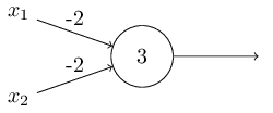
input 00 -> (−2)∗0+(−2)∗0+3= 3 -> output: 3
input 11 -> (−2)∗1+(−2)∗1+3=-1 -> output: -1

sigmoid: This shape is a smoothed out version of a step function.

output would be 1 or 0 depending on whether w⋅x+b was positive or negative

28 by 28 pixel images of scanned handwritten digits, and so the input layer contains 784=28×28

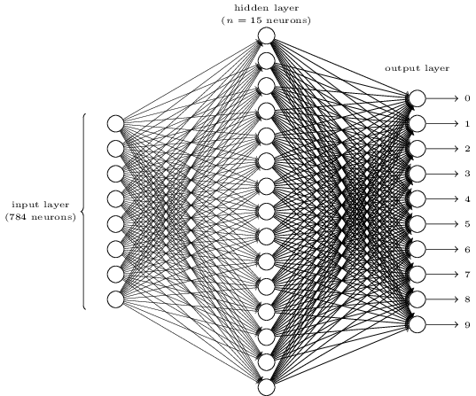
Supposing the neural network functions in this way, we can give a plausible explanation for why it’s better to have 10 outputs from the network, rather than 4. If we had 4 outputs, then the first output neuron would be trying to decide what the most significant bit of the digit was. And there’s no easy way to relate that most significant bit to simple shapes like those shown above. It’s hard to imagine that there’s any good historical reason the component shapes of the digit will be closely related to (say) the most significant bit in the output.

Download and Setup @

sudo pip install --upgrade https://storage.googleapis.com/tensorflow/linux/cpu/tensorflow-0.8.0-cp27-none-linux_x86_64.whl
python -c 'import os; import inspect; import tensorflow; print(os.path.dirname(inspect.getfile(tensorflow)))'
/usr/local/lib/python2.7/dist-packages/tensorflow

# Using 'python -m' to find the program in the python search path:
$ python -m tensorflow.models.image.mnist.convolutional
Extracting data/train-images-idx3-ubyte.gz
Extracting data/train-labels-idx1-ubyte.gz
Extracting data/t10k-images-idx3-ubyte.gz
Extracting data/t10k-labels-idx1-ubyte.gz
...etc...

# You can alternatively pass the path to the model program file to the python
# interpreter (make sure to use the python distribution you installed
# TensorFlow to, for example, .../python3.X/... for Python 3).
$ python /usr/local/lib/python2.7/dist-packages/tensorflow/models/image/mnist/convolutional.py
...

机器学习（一）：生成学习算法Generative Learning algorithms - zjgtan - 博客园

Rectifier (neural networks) @

In the context of artificial neural networks, the rectifier is an activation function defined as

\[f(x) = \max(0, x)\]

where x is the input to a neuron. This is also known as a ramp function, and it is analogous to half-wave rectification in electrical engineering. This activation function has been argued to be more biologically plausible than the widely used logistic sigmoid (which is inspired by probability theory; see logistic regression) and its more practical counterpart, the hyperbolic tangent. The rectifier is, as of 2015, the most popular activation function for deep neural networks.

Plot of the rectifier (blue) and softplus (green) functions near x = 0.

A unit employing the rectifier is also called a rectified linear unit (ReLU).

A smooth approximation to the rectifier is the analytic function

\[f(x) = \ln(1 + e^x)\]

which is called the softplus function. The derivative of softplus is $f'(x) = e^x / (e^x+1) = 1 / (1 + e^{-x})$, i.e. the logistic function.

Rectified linear units find applications in computer vision, and speech recognition using deep neural nets.

UFLDL 教程 - Ufldl @

如果选择 f(z) = 1/(1+(-z)) ，也就是 sigmoid 函数，那么它的导数就是 f’(z) = f(z) (1-f(z)) （如果选择 tanh 函数，那它的导数就是 f’(z) = 1- (f(z))^2 ，你可以根据 sigmoid（或 tanh）函数的定义自行推导这个等式。

Qix/dl.md at master · ty4z2008/Qix

CSC2515F : lectures

CIE 1931 color space - Wikipedia, the free encyclopedia @

Lab color space - Wikipedia, the free encyclopedia @: A Lab color space is a color-opponent space with dimension L for lightness and a and b for the color-opponent dimensions, based on nonlinearly compressed (e.g. CIE XYZ color space) coordinates.

Minimum distance estimation - Wikipedia, the free encyclopedia

余凯在清华的讲座笔记 - huangbo10 的专栏 - 博客频道 - CSDN.NET

Learning and neural networks - Wikiversity

Hacker’s guide to Neural Networks @

Andrej Karpathy Academic Website

这里有更完整的代码和 materials。

More materials

My personal experience with Neural Networks is that everything became much clearer when I started ignoring full-page, dense derivations of backpropagation equations and just started writing code. Thus, this tutorial will contain very little math (I don’t believe it is necessary and it can sometimes even obfuscate simple concepts).

Chapter 1: Real-valued Circuits @

看成门电路，不只是 {0, 1}，更是 real values 在线路上 flow。除了 AND，OR，NOT 还有 binary gates 如 * (multiply), + (add), max， unary gates 比如 exp，等等。

Base Case: Single Gate in the Circuit @

base case，一个简单的 single gate in the circuit。进行 f(x,y) = x*y 的操作， javascript 代码如下：

var forwardMultiplyGate = function(x, y) {
  return x * y;
};
forwardMultiplyGate(-2, 3); // returns -6. Exciting.

我们的目标是让它的输出变大。这里有三个策略：

Strategy #1: Random Local Search @

随机在周围找点，然后看是否更大，更大就记录下来。

// circuit with single gate for now
var forwardMultiplyGate = function(x, y) { return x * y; };
var x = -2, y = 3; // some input values

// try changing x,y randomly small amounts and keep track of what works best
var tweak_amount = 0.01;
var best_out = -Infinity;
var best_x = x, best_y = y;
for(var k = 0; k < 100; k++) {
  var x_try = x + tweak_amount * (Math.random() * 2 - 1); // tweak x a bit
  var y_try = y + tweak_amount * (Math.random() * 2 - 1); // tweak y a bit
  var out = forwardMultiplyGate(x_try, y_try);
  if(out > best_out) {
    // best improvement yet! Keep track of the x and y
    best_out = out;
    best_x = x_try, best_y = y_try;
  }
}

Stategy #2: Numerical Gradient @

求出数值梯度。∂f(x,y)/∂x = (f(x+h,y)−f(x,y))/h，这里的 h 是一个 tweak amount。Javascript 代码如下：

var x = -2, y = 3;
var out = forwardMultiplyGate(x, y); // -6
var h = 0.0001;

// 对 x 的偏导
var xph = x + h; // -1.9999
var out2 = forwardMultiplyGate(xph, y); // -5.9997
var x_derivative = (out2 - out) / h; // 3.0

// 对 y 的偏导
var yph = y + h; // 3.0001
var out3 = forwardMultiplyGate(x, yph); // -6.0002
var y_derivative = (out3 - out) / h; // -2.0

// 指定 stepsize，给输入添加一点 tweak amount，
// 得到新的输出，而且输出值真的更大一些！
var step_size = 0.01;
var out = forwardMultiplyGate(x, y); // before: -6
x = x + step_size * x_derivative; // x becomes -1.97
y = y + step_size * y_derivative; // y becomes 2.98
var out_new = forwardMultiplyGate(x, y); // -5.87! exciting.

The derivative with respect to some input can be computed by tweaking that input by a small amount and observing the change on the output value.

Strategy #3: Analytic Gradient @

分析导数。相比数值导数，这个需要一点数学知识。好处是可以得到 exact 导数，而且计算量小。

The analytic derivative requires no tweaking of the inputs. It can be derived using mathematics (calculus).

Javascript 代码：

var x = -2, y = 3;
var out = forwardMultiplyGate(x, y); // before: -6
var x_gradient = y; // by our complex mathematical derivation above
var y_gradient = x;

var step_size = 0.01;
x += step_size * x_gradient; // -2.03
y += step_size * y_gradient; // 2.98
var out_new = forwardMultiplyGate(x, y); // -5.87. Higher output! Nice.

小结。Lets recap what we have learned: @

INPUT: We are given a circuit, some inputs and compute an output value.
OUTPUT: We are then interested finding small changes to each input (independently) that would make the output higher.
Strategy #1: One silly way is to randomly search for small pertubations of the inputs and keep track of what gives the highest increase in output.
Strategy #2: We saw we can do much better by computing the gradient. Regardless of how complicated the circuit is, the numerical gradient is very simple (but relatively expensive) to compute. We compute it by probing the circuit’s output value as we tweak the inputs one at a time.
Strategy #3: In the end, we saw that we can be even more clever and analytically derive a direct expression to get the analytic gradient. It is identical to the numerical gradient, it is fastest by far, and there is no need for any tweaking.

Recursive Case: Circuits with Multiple Gates @

f(x,y,z) = (x+y)*z，直接看代码吧，看解释不如看代码。

分三个过程：

forword，计算输出： @

var forwardMultiplyGate = function(a, b) {
  return a * b;
};
var forwardAddGate = function(a, b) {
  return a + b;
};
var forwardCircuit = function(x,y,z) {
  var q = forwardAddGate(x, y);
  var f = forwardMultiplyGate(q, z);
  return f;
};

var x = -2, y = 5, z = -4;
var f = forwardCircuit(x, y, z); // output is -12

backward，反向传播，计算偏导（决定了输入的更新）： @

// initial conditions
var x = -2, y = 5, z = -4;
var q = forwardAddGate(x, y); // q is 3
var f = forwardMultiplyGate(q, z); // output is -12

// gradient of the MULTIPLY gate with respect to its inputs
// wrt is short for "with respect to"
var derivative_f_wrt_z = q; // 3
var derivative_f_wrt_q = z; // -4

// derivative of the ADD gate with respect to its inputs
var derivative_q_wrt_x = 1.0;
var derivative_q_wrt_y = 1.0;

// chain rule
var derivative_f_wrt_x = derivative_q_wrt_x * derivative_f_wrt_q; // -4
var derivative_f_wrt_y = derivative_q_wrt_y * derivative_f_wrt_q; // -4

forward，根据反向传播得到的偏导，更新输入，再计算输出： @

// final gradient, from above: [-4, -4, 3]
var gradient_f_wrt_xyz = [derivative_f_wrt_x, derivative_f_wrt_y, derivative_f_wrt_z]

// let the inputs respond to the force/tug:
var step_size = 0.01;
x = x + step_size * derivative_f_wrt_x; // -2.04
y = y + step_size * derivative_f_wrt_y; // 4.96
z = z + step_size * derivative_f_wrt_z; // -3.97

// Our circuit now better give higher output:
var q = forwardAddGate(x, y); // q becomes 2.92
var f = forwardMultiplyGate(q, z); // output is -11.59, up from -12! Nice!

发现确实输出值确实加大了。

理解到了这里，你就明白了反向传播到底是在干嘛。

小结。Lets recap once again what we learned:

In the previous chapter we saw that in the case of a single gate (or a single expression), we can derive the analytic gradient using simple calculus. We interpreted the gradient as a force, or a tug on the inputs that pulls them in a direction which would make this gate’s output higher.
In case of multiple gates everything stays pretty much the same way: every gate is hanging out by itself completely unaware of the circuit it is embedded in. Some inputs come in and the gate computes its output and the derivate with respect to the inputs. The only difference now is that suddenly, something can pull on this gate from above. That’ s the gradient of the final circuit output value with respect to the ouput this gate computed. It is the circuit asking the gate to output higher or lower numbers, and with some force. The gate simply takes this force and multiplies it to all the forces it computed for its inputs before (chain rule). This has the desired effect:
If a gate experiences a strong positive pull from above, it will also pull harder on its own inputs, scaled by the force it is experiencing from above
And if it experiences a negative tug, this means that circuit wants its value to decrease not increase, so it will flip the force of the pull on its inputs to make its own output value smaller.

A nice picture to have in mind is that as we pull on the circuit’s output value at the end, this induces pulls downward through the entire circuit, all the way down to the inputs.

就是说我们在输出端施加一个力，这个力能够返回去作用到电路的输入。

Patterns in the “backward” flow @

说的就是 + 和 * 反向传播的规律。（对 + 而言，是把 sigma 直接分散回去；对 * 而言，是交换输入值。）

Example: Single Neuron @

f(x,y,a,b,c) = σ(ax+by+c)。

sigmoid 函数很符合显示规律，是一个 sigmoid 形状（“S” 形）。但 “S” 形的函数多了去，为什么要用 sigmoid = 1/(1+e^(-x))？因为这个函数很方便计算导数。而且，在神经网络中，不仅仅是 sigmoid 函数的导数是 sig’(x) = sig(x)(1-sig(x))，更是 sig(x) 在 forward 已经算过了！也就是说 sigmoid 函数求导数，计算任务的负担和 x(1-x) 一样……是不是很赞？！

线路中每条线其实有两样数值于此相关，一个是 forward 时传递的输入值，一个是 backward 时反向传递的 gradients。我们先创建一个 Unit 单元来存储电路中的 wire 的 input value 和 weights：

// every Unit corresponds to a wire in the diagrams
var Unit = function(value, grad) {
  // value computed in the forward pass
  this.value = value;
  // the derivative of circuit output w.r.t this unit, computed in backward pass
  this.grad = grad;
}

除了 unit 我们还要有一个 +，一个 * 和一个 sig (sigmoid)。

multiplyGate @

var multiplyGate = function(){ };
multiplyGate.prototype = {
  forward: function(u0, u1) {
    // store pointers to input Units u0 and u1 and output unit utop
    this.u0 = u0;
    this.u1 = u1;
    this.utop = new Unit(u0.value * u1.value, 0.0);
    return this.utop;
  },
  backward: function() {
    // take the gradient in output unit and chain it with the
    // local gradients, which we derived for multiply gate before
    // then write those gradients to those Units.
    this.u0.grad += this.u1.value * this.utop.grad;
    this.u1.grad += this.u0.value * this.utop.grad;
  }
}

addGate @

var addGate = function(){ };
addGate.prototype = {
  forward: function(u0, u1) {
    this.u0 = u0;
    this.u1 = u1; // store pointers to input units
    this.utop = new Unit(u0.value + u1.value, 0.0);
    return this.utop;
  },
  backward: function() {
    // add gate. derivative wrt both inputs is 1
    this.u0.grad += 1 * this.utop.grad;
    this.u1.grad += 1 * this.utop.grad;
  }
}

sigmoidGate @

var sigmoidGate = function() {
    // helper function
    this.sig = function(x) { return 1 / (1 + Math.exp(-x)); };
};
sigmoidGate.prototype = {
    forward: function(u0) {
        this.u0 = u0;
        this.utop = new Unit(this.sig(this.u0.value), 0.0);
        return this.utop;
    },
    backward: function() {
        var s = this.sig(this.u0.value);
        this.u0.grad += (s * (1 - s)) * this.utop.grad;
    }
}

然后就可以拿来算了：

forward @

// create input units
var a = new Unit(1.0, 0.0);
var b = new Unit(2.0, 0.0);
var c = new Unit(-3.0, 0.0);
var x = new Unit(-1.0, 0.0);
var y = new Unit(3.0, 0.0);

// create the gates
var mulg0 = new multiplyGate();
var mulg1 = new multiplyGate();
var addg0 = new addGate();
var addg1 = new addGate();
var sg0 = new sigmoidGate();

// do the forward pass
var forwardNeuron = function() {
  ax = mulg0.forward(a, x); // a*x = -1
  by = mulg1.forward(b, y); // b*y = 6
  axpby = addg0.forward(ax, by); // a*x + b*y = 5
  axpbypc = addg1.forward(axpby, c); // a*x + b*y + c = 2
  s = sg0.forward(axpbypc); // sig(a*x + b*y + c) = 0.8808
};
forwardNeuron();

console.log('circuit output: ' + s.value); // prints 0.8808

backward @

s.grad = 1.0;
sg0.backward(); // writes gradient into axpbypc
addg1.backward(); // writes gradients into axpby and c
addg0.backward(); // writes gradients into ax and by
mulg1.backward(); // writes gradients into b and y
mulg0.backward(); // writes gradients into a and x

forward @

var step_size = 0.01;
a.value += step_size * a.grad; // a.grad is -0.105
b.value += step_size * b.grad; // b.grad is 0.315
c.value += step_size * c.grad; // c.grad is 0.105
x.value += step_size * x.grad; // x.grad is 0.105
y.value += step_size * y.grad; // y.grad is 0.210

forwardNeuron();
console.log('circuit output after one backprop: ' + s.value); // prints 0.8825

我们还可以检验一下 bp 算出来的 grad 是否正确，

var forwardCircuitFast = function(a,b,c,x,y) {
  return 1/(1 + Math.exp( - (a*x + b*y + c)));
};
var a = 1, b = 2, c = -3, x = -1, y = 3;
var h = 0.0001;
var a_grad = (forwardCircuitFast(a+h,b,c,x,y) - forwardCircuitFast(a,b,c,x,y))/h;
var b_grad = (forwardCircuitFast(a,b+h,c,x,y) - forwardCircuitFast(a,b,c,x,y))/h;
var c_grad = (forwardCircuitFast(a,b,c+h,x,y) - forwardCircuitFast(a,b,c,x,y))/h;
var x_grad = (forwardCircuitFast(a,b,c,x+h,y) - forwardCircuitFast(a,b,c,x,y))/h;
var y_grad = (forwardCircuitFast(a,b,c,x,y+h) - forwardCircuitFast(a,b,c,x,y))/h;

Becoming a Backprop Ninja @

// 这种情况是简单的
var x = a + b + c;
var da = 1.0 * dx; var db = 1.0 * dx; var dc = 1.0 * dx;

// 这种情况呢？
var x = a * a;
var da = //???

// 可以做如下考虑
var da = a * dx; // gradient into a from first branch
da += a * dx; // and add on the gradient from the second branch

// short form instead is:
var da = 2 * a * dx;

还有更难的例子。

还有，ReLU 呢？

var x = Math.max(a, 0)
// backprop through this gate will then be:
var da = a > 0 ? 1.0 * dx : 0.0;

“Maybe this is not immediately obvious, but this machinery is a powerful hammer for Machine Learning.”

Chapter 2: Machine Learning

附录

这是我当时查看了的一些资料，留作笔记。

Multilayer perceptron

A multilayer perceptron (MLP) is a feedforward artificial neural network model that maps sets of input data onto a set of appropriate outputs. An MLP consists of multiple layers of nodes in a directed graph, with each layer fully connected to the next one. Except for the input nodes, each node is a neuron (or processing element) with a nonlinear activation function. MLP utilizes a supervised learning technique called backpropagation for training the network. MLP is a modification of the standard linear perceptron and can distinguish data that are not linearly separable.

The term “multilayer perceptron” often causes confusion. It is argued the model is not a single perceptron that has multiple layers. Rather, it contains many perceptrons that are organised into layers, leading some to believe that a more fitting term might therefore be “multilayer perceptron network”. Moreover, these “perceptrons” are not really perceptrons in the strictest possible sense, as true perceptrons are a special case of artificial neurons that use a threshold activation function such as the Heaviside step function, whereas the artificial neurons in a multilayer perceptron are free to take on any arbitrary activation function. Consequently, whereas a true perceptron performs binary classification, a neuron in a multilayer perceptron is free to either perform classification or regression, depending upon its activation function.

Artificial neural network

In machine learning and cognitive science, artificial neural networks (ANNs) are a family of models inspired by biological neural networks (the central nervous systems of animals, in particular the brain) and are used to estimate or approximate functions that can depend on a large number of inputs and are generally unknown. Artificial neural networks are generally presented as systems of interconnected “neurons” which exchange messages between each other. The connections have numeric weights that can be tuned based on experience, making neural nets adaptive to inputs and capable of learning.

Like other machine learning methods - systems that learn from data - neural networks have been used to solve a wide variety of tasks that are hard to solve using ordinary rule-based programming, including computer vision and speech recognition.

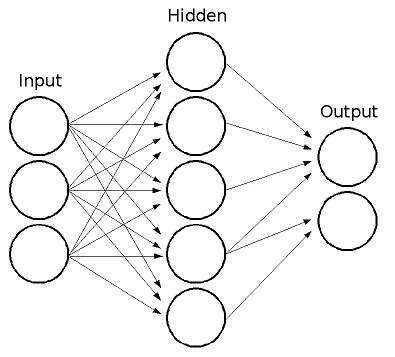
Multi-Layer Perceptrons (MLP)

We can classify people in this problem using a single layer perceptron

A perceptron learns by a trial and error like method. It takes the input such as our math and Star Trek scores and outputs what it thinks the persons job is. Based on how far off its guess is, we will adjust each weight slowly to compensate. This will move its answers over time to be more accurate

A Multilayer perceptron is two single layer perceptrons stacked on top of each other with typically a sigmoidal activation function between the two layers to make the numbers more crisp.

All the neurons in MLP are similar. Each of them has several input links (it takes the output values from several neurons in the previous layer as input) and several output links (it passes the response to several neurons in the next layer). The values retrieved from the previous layer are summed up with certain weights, individual for each neuron, plus the bias term. The sum is transformed using the activation function $f$ that may be also different for different neurons.

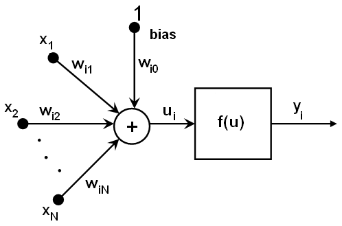
In other words, given the outputs $x_j$ of the layer $n$ , the outputs $y_i$ of the layer $n+1$ are computed as:

\[ u_i = \sum _j (w^{n+1}_{i,j}*x_j) + w^{n+1}_{i,bias} \]

\[ y_i = f(u_i) \]

Different activation functions may be used. ML implements three standard functions:

Identity function ( CvANN_MLP::IDENTITY ): $f(x)=x$
Symmetrical sigmoid⁷ ( CvANN_MLP::SIGMOID_SYM ): $f(x)=\beta*(1-e^{-\alpha x})/(1+e^{-\alpha x} )$, which is the default choice for MLP. The standard sigmoid with $\beta =1$, $\alpha =1$ is shown below: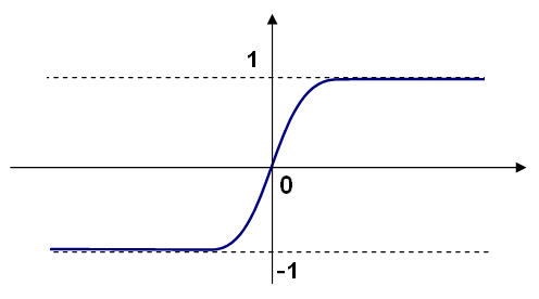
Gaussian function ( CvANN_MLP::GAUSSIAN ): $f(x)=\beta e^{-\alpha x^2}$, which is not completely supported at the moment.

In ML, all the neurons have the same activation functions, with the same free parameters ($\alpha$, $\beta$) that are specified by user and are not altered by the training algorithms.

So, the whole trained network works as follows:

Take the feature vector as input. The vector size is equal to the size of the input layer.
Pass values as input to the first hidden layer .
Compute outputs of the hidden layer using the weights and the activation functions.
Pass outputs further downstream until you compute the output layer.

So, to compute the network, you need to know all the weights $w^{n+1}_{i,j}$. The weights are computed by the training algorithm. The algorithm takes a training set, multiple input vectors with the corresponding output vectors, and iteratively adjusts the weights to enable the network to give the desired response to the provided input vectors.

The larger the network size (the number of hidden layers and their sizes) is, the more the potential network flexibility is. The error on the training set could be made arbitrarily small. But at the same time the learned network also “learns” the noise present in the training set, so the error on the test set usually starts increasing after the network size reaches a limit. Besides, the larger networks are trained much longer than the smaller ones, so it is reasonable to pre-process the data, using PCA::operator() or similar technique, and train a smaller network on only essential features.

Another MLP feature is an inability to handle categorical data as is. However, there is a workaround. If a certain feature in the input or output (in case of $n$-class classifier for $n>2$) layer is categorical and can take $M>2$ different values, it makes sense to represent it as a binary tuple of $M$ elements, where the $i$-th element is 1 if and only if the feature is equal to the $i$-th value out of $M$ possible. It increases the size of the input/output layer but speeds up the training algorithm convergence and at the same time enables “fuzzy” values of such variables, that is, a tuple of probabilities instead of a fixed value.

ML implements two algorithms for training MLP’s. The first algorithm is a classical random sequential back-propagation⁸ algorithm. The second (default) one is a batch RPROP algorithm.

CvANN_MLP

CvANN_MLP::create

Constructs MLP with the specified topology.

Unlike many other models in ML that are constructed and trained at once, in the MLP model these steps are separated. First, a network with the specified topology is created using the non-default constructor or the method CvANN_MLP::create(). All the weights are set to zeros. Then, the network is trained using a set of input and output vectors. The training procedure can be repeated more than once, that is, the weights can be adjusted based on the new training data.

void CvANN_MLP::create( const Mat& layerSizes,
                        int activateFunc=CvANN_MLP::SIGMOID_SYM,
                        double fparam1=0,
                        double fparam2=0 );

void CvANN_MLP::create( const CvMat* layerSizes,
                        int activateFunc=CvANN_MLP::SIGMOID_SYM,
                        double fparam1=0,
                        double fparam2=0 );

Parameters

layerSizes – Integer vector specifying the number of neurons in each layer including the input and output layers.
activateFunc – Parameter specifying the activation function for each neuron: one of CvANN_MLP::IDENTITY, CvANN_MLP::SIGMOID_SYM, and CvANN_MLP::GAUSSIAN.
fparam1 – Free parameter of the activation function, $\alpha$. See the formulas in the introduction section.
fparam2 – Free parameter of the activation function, $\beta$. See the formulas in the introduction section.

CvANN_MLP::train

Trains/updates MLP.

int CvANN_MLP::train( const Mat& inputs,
                      const Mat& outputs,
                      const Mat& sampleWeights,
                      const Mat& sampleIdx=Mat(),
                      CvANN_MLP_TrainParams params=CvANN_MLP_TrainParams(),
                      int flags=0 );

int CvANN_MLP::train( const CvMat* inputs,
                      const CvMat* outputs,
                      const CvMat* sampleWeights,
                      const CvMat* sampleIdx=0,
                      CvANN_MLP_TrainParams params=CvANN_MLP_TrainParams(),
                      int flags=0 );

inputs – Floating-point matrix of input vectors, one vector per row.
outputs – Floating-point matrix of the corresponding output vectors, one vector per row.
sampleWeights – (RPROP only) Optional floating-point vector of weights for each sample. Some samples may be more important than others for training. You may want to raise the weight of certain classes to find the right balance between hit-rate and false-alarm rate, and so on.
sampleIdx – Optional integer vector indicating the samples (rows of inputs and outputs) that are taken into account. params – Training parameters. See the CvANN_MLP_TrainParams description.
flags
- Various parameters to control the training algorithm. A combination of the following parameters is possible:
  - UPDATE_WEIGHTS Algorithm updates the network weights, rather than computes them from scratch. In the latter case the weights are initialized using the Nguyen-Widrow algorithm.
  - NO_INPUT_SCALE Algorithm does not normalize the input vectors. If this flag is not set, the training algorithm normalizes each input feature independently, shifting its mean value to 0 and making the standard deviation equal to 1. If the network is assumed to be updated frequently, the new training data could be much different from original one. In this case, you should take care of proper normalization.
  - NO_OUTPUT_SCALE Algorithm does not normalize the output vectors. If the flag is not set, the training algorithm normalizes each output feature independently, by transforming it to the certain range depending on the used activation function.

CvANN_MLP::predict

Predicts responses for input samples.

float CvANN_MLP::predict( const Mat& inputs,
                          Mat& outputs) const;

float CvANN_MLP::predict( const CvMat* inputs,
                          CvMat* outputs) const;

If you are using the default cvANN_MLP::SIGMOID_SYM activation function with the default parameter values fparam1=0 and fparam2=0 then the function used is y = 1.7159tanh(2/3 x), so the output will range from [-1.7159, 1.7159], instead of [0,1].

int CvANN_MLP::get_layer_count()

const CvMat* CvANN_MLP::get_layer_sizes();

double *CvANN_MLP::get_weights( int layer );

An example

#include <opencv2/core/core.hpp>
#include <opencv2/highgui/highgui.hpp>
#include <opencv2/ml/ml.hpp>
#include <iostream>
#include <string>

using namespace std;
using namespace cv;

int main()
{
    CvANN_MLP bp;

    //  CvANN_MLP_TrainParams::CvANN_MLP_TrainParams()
    //  {
    //      term_crit = cvTermCriteria(
    //              CV_TERMCRIT_ITER + CV_TERMCRIT_EPS, 1000, 0.01 );
    //      train_method = RPROP;
    //      bp_dw_scale = bp_moment_scale = 0.1;
    //      rp_dw0 = 0.1; rp_dw_plus = 1.2; rp_dw_minus = 0.5;
    //      rp_dw_min = FLT_EPSILON; rp_dw_max = 50.;
    //  }
    CvANN_MLP_TrainParams params;

    // CvANN_MLP_TrainParams::BACKPROP The back-propagation algorithm.
    // CvANN_MLP_TrainParams::RPROP The RPROP algorithm.
    params.train_method = CvANN_MLP_TrainParams::BACKPROP;

    // Strength of the weight gradient term. The recommended value is about 0.1
    // params.bp_dw_scale = 0.1;

    // Strength of the momentum term (the difference between weights on the 2
    // previous iterations). This parameter provides some inertia to smooth the
    // random fluctuations of the weights. It can vary from 0 (the feature is
    // disabled) to 1 and beyond. The value 0.1 or so is good enough
    // params.bp_moment_scale = 0.1;

    // Initial value \Delta_0 of update-values \Delta_{ij}.
    // params.rp_dw0 = 0.1;

    // Increase factor \eta^+. It must be >1.
    // params.rp_dw_plus = 1.2;

    // Decrease factor \eta^-. It must be <1.
    // params.rp_dw_minus = 0.5;

    // Update-values lower limit \Delta_{min}. It must be positive.
    // params.rp_dw_min = FLT_EPSILON;

    // Update-values upper limit \Delta_{max}. It must be >1.
    // params.rp_dw_max = 50.;

    // void CvANN_MLP::create(const Mat& layerSizes,
    //                        int activateFunc=CvANN_MLP::SIGMOID_SYM,
    //                        double fparam1=0,
    //                        double fparam2=0 )
    // * layerSizes – #neurons in each layer including the input/output layers
    // * activateFunc – activation function for each neuron
    //      CvANN_MLP::IDENTITY
    //      CvANN_MLP::SIGMOID_SYM
    //      CvANN_MLP::GAUSSIAN
    // * fparam1 – Free parameter of the activation function, \alpha
    // * fparam2 – Free parameter of the activation function, \beta
    Mat layerSizes=(Mat_<int>(1,5) << 5,2,2,2,5);
    bp.create( layerSizes, CvANN_MLP::SIGMOID_SYM );

    // int CvANN_MLP::train(
    //      const Mat& inputs,
    //      const Mat& outputs,
    //      const Mat& sampleWeights,
    //      const Mat& sampleIdx=Mat(),
    //      CvANN_MLP_TrainParams params=CvANN_MLP_TrainParams()
    //      int flags=0 )

    float trainingData[3][5] = {
        {   1,   2,   3,   4,  5 },
        { 111, 112, 113, 114, 115},
        {  21,  22,  23,  24,  25},
    };
    Mat trainingDataMat(3, 5, CV_32FC1, trainingData);

    float labels[3][5] = {
        { 0, 0, 0, 0, 0 },
        { 0, 0, 0, 0, 0 },
        { 1, 1, 1, 1, 1 },
    };
    Mat labelsMat(3, 5, CV_32FC1, labels);

    bp.train( trainingDataMat, labelsMat, Mat(), Mat(), params );

    // Data for visual representation
    int width = 512, height = 512;
    Mat image = Mat::zeros( height, width, CV_8UC3 );
    Vec3b green( 0, 255, 0 ), blue ( 255, 0, 0 );

    // Show the decision regions given by the SVM
    for ( int i = 0; i < image.rows; ++i ) {
        for ( int j = 0; j < image.cols; ++j ) {
            Mat sampleMat = (Mat_<float>(1,5) << i,j,0,0,0);
            Mat responseMat;
            bp.predict( sampleMat, responseMat );
            float *p = responseMat.ptr<float>(0);
            float response = 0.0f;
            for( int k=0; k < 5; k++ ) {
                response += p[k];
            }
            if ( response > 2 ) {
                image.at<Vec3b>(j, i)  = green;
            } else {
                image.at<Vec3b>(j, i)  = blue;
            }
        }
    }

    // Show the training data
    circle( image, Point(501,  10), 5, Scalar(  0,   0,   0), -1, 8 );
    circle( image, Point(255,  10), 5, Scalar(255, 255, 255), -1, 8 );
    circle( image, Point(501, 255), 5, Scalar(255, 255, 255), -1, 8 );
    circle( image, Point( 10, 501), 5, Scalar(255, 255, 255), -1, 8 );

    imwrite("result.png", image);       // save the image
    imshow("BP Simple Example", image); // show it to the user
    cvWaitKey(0);
}

参考文献

10.10. shutil — High-level file operations — Python 2.7.11 documentation ↩
Tutorial — Theano 0.8.0 documentation.↩
see NumPy refresher — Theano 0.8.0 documentation.↩
Derivatives in Theano — Theano 0.8.0 documentation.↩
Conditions — Theano 0.8.0 documentation.↩
NAND gate - Wikipedia, the free encyclopedia.↩
A sigmoid function is a mathematical function having an “S” shape (sigmoid curve).

单调递增的非线性函数，无限次可微。当且仅当权值较大时可以逼近阈值函数，当权值较小时逼线性函数。

Besides the logistic function ($f(x) = \frac{L}{1 + \mathrm e^{-k(x-x_0)}}$), sigmoid functions include the ordinary arctangent, the hyperbolic tangent, the Gudermannian function, and the error function ($\operatorname{erf}(x) = \frac{2}{\sqrt\pi}\int_0^x e^{-t^2}\,\mathrm dt$), but also the generalised logistic function and algebraic functions like $f(x)=\tfrac{x}{\sqrt{1+x^2}}$.

↩
Backpropagation, an abbreviation for “backward propagation of errors”, is a common method of training artificial neural networks used in conjunction with an optimization method such as gradient descent. The method calculates the gradient of a loss function with respect to all the weights in the network. The gradient is fed to the optimization method which in turn uses it to update the weights, in an attempt to minimize the loss function.

BP 算法就是通过迭代优化网络的权值使得输出与输入之间的实际映射关系与所期望的映射关系一致，采用梯度下降算法通过调整各层权值求目标函数最小化。

Backpropagation requires a known, desired output for each input value in order to calculate the loss function gradient. It is therefore usually considered to be a supervised learning method, although it is also used in some unsupervised networks such as autoencoders. It is a generalization of the delta rule to multi-layered feedforward networks, made possible by using the chain rule to iteratively compute gradients for each layer. Backpropagation requires that the activation function used by the artificial neurons (or “nodes”) be differentiable.

Since backpropagation uses the gradient descent method, one needs to calculate the derivative of the squared error function with respect to the weights of the network. Assuming one output neuron,[note 2] the squared error function is:

\[E = \tfrac{1}{2}(t - y)^2,\]

where

$E$ is the squared error,

$t$ is the target output for a training sample, and

$y$ is the actual output of the output neuron.

The factor of $\textstyle\frac{1}{2}$ is included to cancel the exponent when differentiating. Later, the expression will be multiplied with an arbitrary learning rate, so that it doesn’t matter if a constant coefficient is introduced now.

For each neuron $j$, its output $o_{j}$ is defined as

\[o_{j} = \varphi(\mbox{net}_{j}) = \varphi\left(\sum_{k=1}^{n}w_{kj}o_k\right).\]

The input $\mbox{net}_{j}$ to a neuron is the weighted sum of outputs o_k of previous neurons. If the neuron is in the first layer after the input layer, the $o_k$ of the input layer are simply the inputs $x_k$ to the network. The number of input units to the neuron is $n$. The variable $w_{ij}$ denotes the weight between neurons $i$ and $j$.

The activation function $\varphi$ is in general non-linear and differentiable. A commonly used activation function is the logistic function:

\[\varphi(z) = \frac{1}{1+e^{-z}}\]

which has a nice derivative of:

\[\frac {\partial\varphi}{\partial z} = \varphi(1-\varphi)\]

Calculating the partial derivative of the error with respect to a weight $w_{ij}$ is done using the chain rule twice:

\[\frac{\partial E}{\partial w_{ij}} = \frac{\partial E}{\partial o_j} \frac{\partial o_j}{\partial\mathrm{net_j}} \frac{\partial \mathrm{net_j}}{\partial w_{ij}}\]

In the last term of the right-hand side of the following, only one term in the sum $\mathrm{net_j}$ depends on $w_{ij}$, so that

\[\frac{\partial \mathrm{net_j}}{\partial w_{ij}} = \frac{\partial}{\partial w_{ij}}\left(\sum_{k=1}^{n}w_{kj}o_k\right) = o_i.\]

If the neuron is in the first layer after the input layer, $o_i$ is just $x_i$. The derivative of the output of neuron $j$ with respect to its input is simply the partial derivative of the activation function (assuming here that the logistic function is used):

\[\frac{\partial o_j}{\partial\mathrm{net_j}} = \frac {\partial}{\partial \mathrm{net_j}}\varphi(\mathrm{net_j}) = \varphi(\mathrm{net_j})(1-\varphi(\mathrm{net_j}))\]

This is the reason why backpropagation requires the activation function to be differentiable.

The first term is straightforward to evaluate if the neuron is in the output layer, because then $o_j = y$ and

\[\frac{\partial E}{\partial o_j} = \frac{\partial E}{\partial y} = \frac{\partial}{\partial y} \frac{1}{2}(t - y)^2 = y - t\]

However, if $j$ is in an arbitrary inner layer of the network, finding the derivative E with respect to $o_j$ is less obvious.

Considering $E$ as a function of the inputs of all neurons $L = {u, v, \dots, w}$ receiving input from neuron $j$,

\[\frac{\partial E(o_j)}{\partial o_j} = \frac{\partial E(\mathrm{net}_u, \mathrm{net}_v, \dots, \mathrm{net}_w)}{\partial o_j}\]

and taking the total derivative with respect to $o_j$, a recursive expression for the derivative is obtained:

\[\frac{\partial E}{\partial o_j} = \sum_{l \in L} \left(\frac{\partial E}{\partial \mathrm{net}_l}\frac{\partial \mathrm{net}_l}{\partial o_j}\right) = \sum_{l \in L} \left(\frac{\partial E}{\partial o_{l}}\frac{\partial o_{l}}{\partial \mathrm{net}_l}w_{jl}\right)\]

Therefore, the derivative with respect to $o_j$ can be calculated if all the derivatives with respect to the outputs $o_l$ of the next layer - the one closer to the output neuron – are known.

Putting it all together:

\[\dfrac{\partial E}{\partial w_{ij}} = \delta_{j} o_{i}\]

with

\[\delta_{j} = \frac{\partial E}{\partial o_j} \frac{\partial o_j}{\partial\mathrm{net_j}} = \begin{cases} (o_{j}-t_{j})\varphi(\mbox{net}_{j})(1-\varphi(\mbox{net}_{j})) & \mbox{if } j \mbox{ is an output neuron,}\\ (\sum_{l\in L} \delta_{l} w_{jl})\varphi(\mbox{net}_{j})(1-\varphi(\mbox{net}_{j})) & \mbox{if } j \mbox{ is an inner neuron.} \end{cases}\]

To update the weight $w_{ij}$ using gradient descent, one must choose a learning rate, $\alpha$. The change in weight, which is added to the old weight, is equal to the product of the learning rate and the gradient, multiplied by -1:

\[\Delta w_{ij} = - \alpha \frac{\partial E}{\partial w_{ij}}\]

The $\textstyle -1$ is required in order to update in the direction of a minimum, not a maximum, of the error function.

For a single-layer network, this expression becomes the Delta Rule. To better understand how backpropagation works, here is an example to illustrate it: The Back Propagation Algorithm, page 20.

Limitations
1. Gradient descent can find the local minimum instead of the global minimum Gradient descent with backpropagation is not guaranteed to global minimum of the error function, but only a local minimum; also, it has trouble crossing plateaus in the error function landscape. This issue, caused by the non-convexity of error functions in neural networks, was long thought to be a major drawback, but in a 2015 review article, Yann LeCun et al. argue that in many practical problems, it isn’t.
2. Backpropagation learning does not require normalization of input vectors; however, normalization could improve performance
A simple neural network with two input units and one output unit:

gradient descent:

↩